Hat Creek ATA - Struggling On

techie wise ;-))

back to main ATA page

Introduction to this web page

This is definitely a work in progress - what ever progress is - as of October 22, 2007 Contents:
- Memo Synopsis
- Beam Forming Simulations
- RF Conversion
- Beam Forming
- Visit to Berkeley Oct 22,2007

Collection of interesting links

- RFI Monitor, Hat Creek 2001
- FCC Table of Frequency Allocations
- RAL Spectrun Management says 1350-1400 MHz (page 31, non-flying?) and 4950-4990 MHz for radio astronomy.
- - really seems to be 1.400 to 1427 GHz solo, 1.610 1.613 shared, 2.690 2.700,4.900 5.000, ... 275-1000 not currently allocated
- RAL ATA Imager Documents
- SETI Diagrams, 1, 2, 3&4, 5&6, DesignGoals, "Effective diameter, 700 meter, Natural weighting", 10 arc sec @ ???
- Transforms
- Sidereal time Greenwich sidereal time and UT1 differ from each other by a constant rate (1.00273790935).
- The GNU Software Radio, Exploring GNU Radio, USRP,
1-650-814-8943, 604 Mariposa, MV,CA HP Agilent 16517A, 16555A
- Sidereal time, local, from Navy
- Right ascension
- Axial tilt
- GPS L1 (1575.42 MHz), L2 (1227.60 MHz)
- (ATA) Memoranda Index
- PFB_32, A 32-pnt Biplex Pipelined Polyphase Filter Bank PBF set up for FFT & finite precision places a noise floor ...
- BEE2, computing platform
- 128 MChannel SETI Spectrometer IBOB diagram .jpg block diagramIBOB is "Internet BreakOut Board" XAUI protocol
-
- celestial mechanics
- M31 - ATA with 42 antennas
-
-
questions
- path gain determination - about 700 paths due to dual polarity
- astronomical orientation
- what is the meaning of latitude of an oblate sphereoid? -
- - a vertical line at say 45 degrees passes through the center of the earth?
- - does not pass through the center of the earth?
- local/universal/GPS time to sidereal, a sidereal second is shorter than a solar second :-|
What a pip - I think we would like to convert local sidereal time and celestial coordinates of target to pointing azimuth and elevation. Then precise pointed location of the "front end" each antenna to variable delays of each data stream.
- My head hurts :-((
- And how do you boresite this whole thing? And tune it up? and keep it tuned?

ATA Memo synopsis - (ATA) Memoranda Index The index also includes links to abstracts in HTML format.

(some ignored as far beyond my capabilities - such as #48 "Proposed Midifications of the ATA Feed Tip")
# remarks-
74
Simulations of Sidelobe Confusion - ATA - estimate dynamic range due to "unpeeled" side lobes. Major sources are Sun, Cas A, Cyg A, etc. If adaptive peeling, max dynamic range of 10^3 (ATA42) and 10^4 (ATA350)
Abstract
73 ATA Correlator - Feb 2007 - two production correlator modules with 8 inputs each (FX8) were installed Jan 2007 - samoled L band analog IF at 800 MHz, probice 100 MHZ input to FX correlator. 61,425 basselines to correlate - 30 KW per tuning - Linux - Progress has been hampered by the fact that the ATA analog to digital, digital dela and fringe rotation system is still in development ... Polyphase filter vs Fourier transform - RF images of M31, M33
Abstract
72 ATA Servo Loop - Nov 2006 - lowest resonate frequency = 3 HZ elevation and azimuth frequencies to avoid in drive. Dirrectly-coupled, incremental encoders step size 9 arc seconds. read @ 19 HZ. Azimuth velocity limited to 3 degree/sec, elevation 1 degree/sec. Kalman filter.
Abstract
71. Cross Correlating Interferometer Beams for Discrimination of Radio ETI Signals
Abstract
70. The ATA Imager Update
Abstract
69. Initial Test Experiments with a Beamformer at the Allen Telescope Array R. Ackermann, August 5, 2005
internal numerically controlled oscillator could not be use to smoothy remove Doppler. They give N,E, Vertical offsets in nanoseconds rather than length.
Abstract
68. Some Thermal Issues Regarding the ATA Node Air System W. J. Welch, March 23, 2005
Interconnecting PVC pipes are burried at 2 foot depth. They feel that the daily swing at that depth is 0.3% of the surface temp. Annual variation is 70 degrees in mid summer and 48 degrees in mid winter. Recommending ambient air to be blown into the pipes for use at the antennas. I presume this is for reducing fiber length and fiber delay time variations. - oh - and also gain variation in the front end receiver !!
Abstract
67. Noise testing of the active and passive baluns for the ATA N. Wadefalk and S. Weinreb, September 7, 2004
- http://astro.uchicago.edu/ursi-comm-J/ursi2005/large-lf-arrays/wadefaul.pdf
Abstract
@ http://astro.berkeley.edu/~greg/ms5498-69.pdf - Wadefalk and Weinreb developed two MMIC (WVA12 and WBA13) devices for the Allen Telescope Array ... include either two or three 0.1um InP HEMT stages tuned to be unconditionally stable when attached to any passive load. The chip size is 2 x 0.7 ~ mm^2. At a 10K operating temperature the WBA12 and 13 have a noise temperature of Tn ~4K and a gain of ~ 25 dB and ~35 dB , respectively, across a 3-11 Ghz band. At 1 GHz, tn ~8 K and gain is 5 dB lower for both. ...
66. Expected Properties of the ATA Antennas W.J. Welch and D.R. DeBoer, July 18, 2004
We find out about the realities of antenna life. Edges defract and don't get fully illuminated. Efficiency is not 100%
Abstract
65. Holography at the ATA G.R. Harp and R.F. Ackermann, March 23, 2004
beyond me -
Abstract
64. Frequency Coverage of the ATA Front-End (Draft) et al, March 19, 2004
Abstract
Details of the "front end", converting 0.5 - 11.5 GHz microwaves to electric current/voltage suitable for Memo 67. above.
63. Notes on Deuterium Detection with the Allen Telescope Array G.C. Bower and M.C.H. Wright, February 13, 2004
Deuterium analog of HI 21 cm line. 92 cm or 327 MHz, not yet detected interstallar. Ratio with HI important constraint on cosmic nucleosynthesis. (Hot off press, Haystack report of April 2007 found/measured it.)
Looks like 500 MHz is a lower practical limit for ATA? 327 MHz is 35 % lower.
Abstract
62. Automatic Interference Mitigation in Large N Correlator Systems Using an Eigenfilter W. L. Urry, January 15, 2004
beyond me -
Abstract
61. Pointing the ATA Dishes G.R. Harp, D.R. DeBoer and G.C. Bower, December 3, 2003
High accuracy than necessary due to beam width helpful for wide angle mosiacs near powerful sources - Cas A - - pointing spec is set at 120 arc seconds, 10% of beam width at 11.2 GHz, just over 1% at HI frequency. Twice that at wind at 15 mph, pointing accuracy unspecified over wind speed of 15 mph. Encoders give readings to 22 arc seconds, final encoders to be 9 arc sec?. Pointing model to help with mechanical imperfections. Difficulty tracking at zenith with Alt/Az mount. Tracking GPS satellites. Morning tracking problems. Hysteresis. Optical pointing at bright stars/planets to observe high frequency dish motions. a movie of tracking Mars a picture sequence of tracking Mars
Abstract
60. Measurements of the Allen Telescope Array Performance as an Interferometer D.R. DeBoer and R.A. Ackermann, November 23, 2003
The ATA antenna has a 3-dB beamwidth of about 3.5degree/GHz. "Phase closure"
Abstract
59. Imaging With a 32-Antenna Allen Telescope Array M.C.H. Wright and G.R. Harp, October 6, 2003
"VLA-D configuration gives about the same resolution and ATA-350.
Abstract
58. J-MIRIAD: Java Wrappers for MIRIAD Methods G.R. Harp and M.C.H. Wright, October 6, 2003
Oh God !!
Abstract
57. Beamforming for Blind Surveys at the ATA G.R. Harp, September 11, 2003
Propose a complex-tapering scheme that gives a large solid angle but with less degradation of beam gain.
Abstract
56. Generation of Unwanted EM Modes in the ATA Feed Dewar W.J. Welch, June 30, 2003
55. Phase Stability of ATA Fiber Optic Cables J.W. Dreher, March 19, 2003
- he feels no particular problem due to slow temperature changes over the buried runs and short vertical runs. "phase up" not too often. something about (Corning) SMF 28e fiber. Single Mode Fiber I can't find any Corning specification of "TCD" - http://199.211.133.239/ptti/1996/Vol%2028_33.pdf says 7 ppm/C - ATA was planned for 1310 nm light, however economics led ATA to adopt 1550 nm lasers.
- Corning SMF-28e+ 'spec' no TCD -
Abstract
- Thermal Coefficient of Delay (TCD) of various fibers in PPM/K, Sumitomo low TCD 0.4 PPM/C
- measurement - http://tycho.usno.navy.mil/ptti/1992/Vol%2024_34.pdf
- cables & glass ATA-techmemo_cbl_temp_stab.pdf - charts not present !!
- Sumitomo fiber ATA-MPPH011.pdf
- I think they are using Corning glass fiber?
54. Tests of an ATA Amplifier and Fiberoptic Link R. Plambeck, J. Cartwright and D. Thornton, January 13, 2003
Frequency response, noise, gain compression of POST Amplifier Module (PAM) through laser, fiber, photodiode.
Prototype ATA "Post Amolifier Module" (PAM s/n 3) and the fiberoptic link (NEC NS85LJ-CC laser, Discovery DSC50S photodiode)
Abstract
53. EPFD Measurements on GPS and Iridium at the RPA N. Imara, January 7, 2003
Known noise sources into the ATA. EPFD is Equivalent Power Flux Density in dB(W/m2 in the reference bandwidth at the radio telescope. Statistical - averaging over days - boxcar integration of 2000 seconds.
Abstract
52. Allen Telescope Array Imaging M. Wright, November 25, 2002
antenna spacings from ~ 10 to 900 m.
"Astronomical imaging well be implemeneted using a digital correlator. For a sparse array, with filling factor 350 x (6m/900m)2 and irreglar antenna spacing, sampling the correlation function, gridding the averaged data, and using FFT algorithms is more efficient than direct imaging."
Serious stuff !! sections are: 1. intro, 2. correlator, 3. data sampling, 4. images, 5. calibration, 5.1 calibration of antenna gains, 5.2 self calibration of antenna gains, 5.3 polarization calibration, 5.4 passband calibration, 6 calibration and imaging architecture, 7. archiving, 8. imaging simulation,
Abstract
51. Customized Beam Forming at the Allen Telescope Array G. R. Harp, August 12, 2002
1. Introduction, 2. Iterative Approach, 3. Beamformer Equation, Beam gain, 4. Single Point Null 5. Multiple Nulls, 6/ Wide Bandwidth Nulls 7. Effects of Phase and Gain Miscalibration, 8. Shaping the beam, 9. Discussion, Control of Coefficient Amplitude, SNR versus k -space Volume, 10. Conclusions Appendix: Some whimsical null patterns
Abstract
50. The Antenna Configuration of the Allen Telescope Array D.C.-J. Bock, January 8, 2003
1. Introduction, 2. Scientific objectives, 3. Configuration optimization, 3.1. Application to the ATA, 4. Analysis, 4.1. The synthesized beam, 4.2. Expected imaging performance, 4.3. Shadowing, 4.4. Tolerance to antenna failures, 4.5. Tolerance to antenna location errors, 5. Discussion, 5.1. Increasing the short spacings, 5.2. Comparison to alternative configuration options, A. The site constraints,
antenna configuration x,y
Abstract
47. Wide Field Imaging Issues for the ATA R. Ekers and G. C. Bower, April 4, 2002
Abstract
46. Broadband Amplitude Calibration of the ATA W. J. Welch and D. C.-J. Bock, March 28, 2002
Abstract
32. Notes on Configuration for the ATA T. T. Helfer, September 18, 2001
Abstract
30. Astronomical Imaging with the ATA - III M. Wright, May 22, 2001
Abstract
21. 350-Antenna Sample Configurations for the Allen Telescope Array D. Bock, March 26, 2001
Abstract
... three sample configurations for the ATA.
1. - randomly distributed acros the central Hat Creek site.
2. - doughnut - 3. maximally filled array
for sidelobe, size, shadowing, sen to extended, connectivity cost.
earth rotation aperture synthesis http://www.merlin.ac.uk/nam/vri/guide.html
& huge
17. Effects of the Sun and RFI on the ATA Offset Gregorian Antenna (Revision history) D. DeBoer and G. Bower, March 1, 2001
Abstract
11. Astronomical Imaging with the Allen Telescope Array - II. M. Wright, November 1, 2000
Abstract
10. The FFT as a Filter Bank. W. L. Urry, October 30, 2000
Abstract
05. The Winds of Hat Creek. D. R. DeBoer, July 11, 2000
They don't seem to mention the wind that knocked over their big antenna. -
Abstract
--. not discussed ?,
  1. the differential heating and subsequent bending of the steel center pole due to sunlight causing mis-location of the antenna elements and focus and subsequent phase errors. This may well be many times the phase errors due to temperature effects in the fiber optics???
  2. How do you {phase-up) the different antennas? how long does it take for 42? 350? each hour when thermally active - like morning is most active?
  3. Does the log periodic antenna have to be re-positioned to be usefully focused at various frequencies?


Apparently understanding the overview of the ATA RF collection scheme is not too tough.
The previous page hinted at everything other than antenna placement and back conversion to RF.
Assuming you have understood the ideas of:

  1. Antenna placement (what pattern on your plot of land is near optimal)
  2. Antenna design and operation (both reflector and receiving elements)
  3. Antenna pointing (both command origination, command chain, servoing)
  4. Focusing of selected frequency onto which part of the receiving elements
  5. Physical offset of the receiving elements due to aiming and warping due to wind and heat
  6. Low noise RF amplifiers
  7. Conversion of RF to fiber optic light at the antenna
  8. Fiber optic delay - length determination and correction of timing of
  9. Conversion of fiber optic light to RF at the central processing facility
moderately well understood, you still have the processing of the various RF streams to do. You have the beginnings necessary to form beams to emulate a normal say 300 (oh yes you should be so lucky) meter steerable antenna.

Lets try to synthesize this fictitious steerable 300 meter from our various RF streams, forming one steered RF stream.

I choose the beam forming method (forming a square law of the power) because I haven't a clue about the alternative method, correlation.

OK - lets begin

The staff and radio astronomer(s) have chosen:

  1. has instructed the software about limitations of each antenna performance
    down, limited tracking, limited frequency, too noisy for some work, ... who knows
  2. Which general "target" to track, and set up the tracking software to point the antennas
    ("Our" actual target needs to be with in some angle of this general target)
  3. Which if not all antennas "we" will use, subsets of antennas can theoretically be used.
    The software is configured for "our" subset of antennas
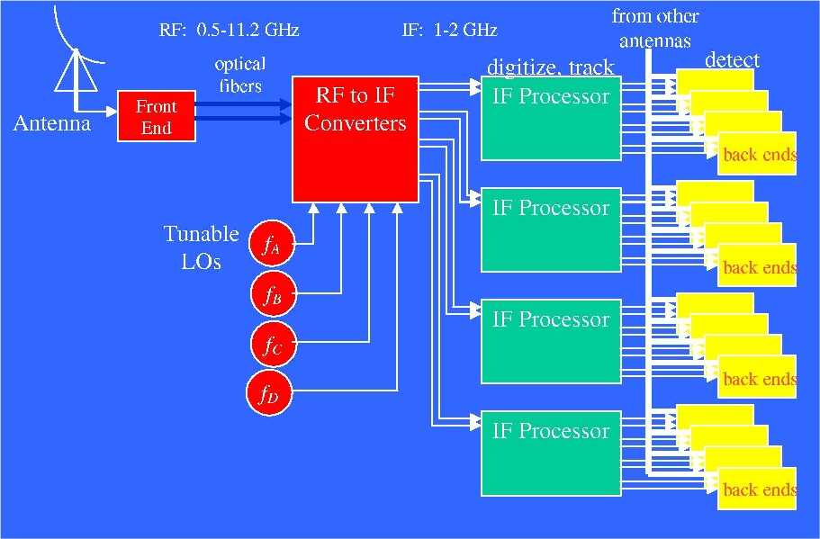
  4. Which ?100? megahertz wide band in the roughly 500 megahertz to 11 gigahertz RF spectrum of the system
    Something/body configures the band limiting filters?, the heterodyning oscillators and post mixing filters
  5. we now have our IF data stream (100 megahertz baseband) from each of the selected, enabled antennas
    Now we choose which of the 16 subchannels per antenna to feed our signal into
    A number of investigators can use our antennas, the common IF is fed into "our" subchannel(s)

To synthesize our 300 meter telescope, we need to get all of these streams into a common phase. The optical telescope people talk of flattening the wave front.

The greater the aperture (distance between the most distant antennas) the smaller the possible beam width for a given frequency (beam width is largely the inverse of the antenna in wavelengths - the more wave lengths, the narrower the beam). A narrow beam enables:
1) better resolution - you can see two distinct points rather than one blur.
2) better signal power, the signal is gathered more efficiently
3) less noise from the ground, earth interference, near by objects in sky :-))
However, since there are a number of discrete antennas, rather than one continuous 300 meter dish, side lobes appear. There is a grand science and art of trying to balance small beam width and minimal side lobes.

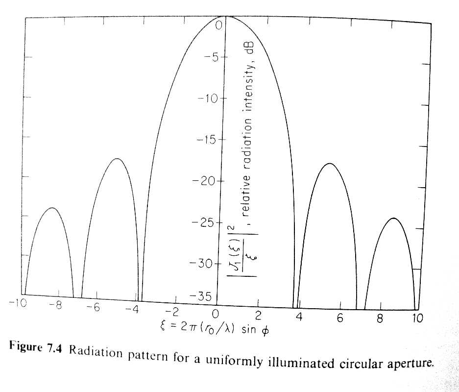
One of the simplest beam forming arrays is the smooth "circular" aperture, implemented as a circular parabola. Nice and simple, all one piece, ...
But even this simple thing has side lobes

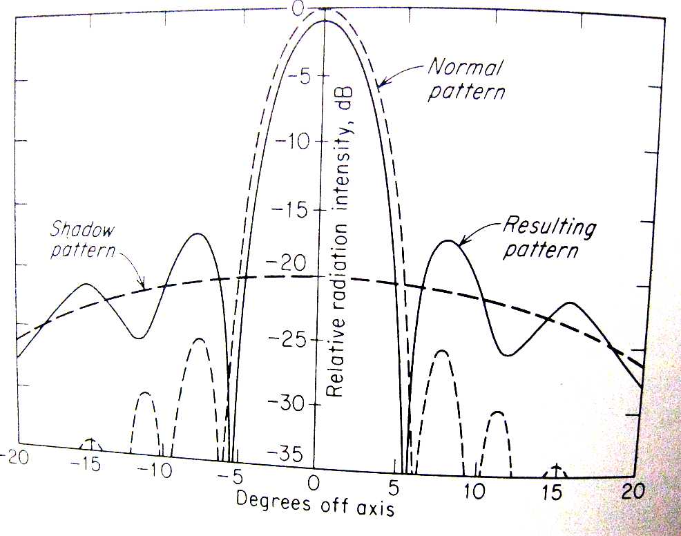
And if you add a feed horn or reflector (usually requiring supports in the beam) the pattern starts getting messy

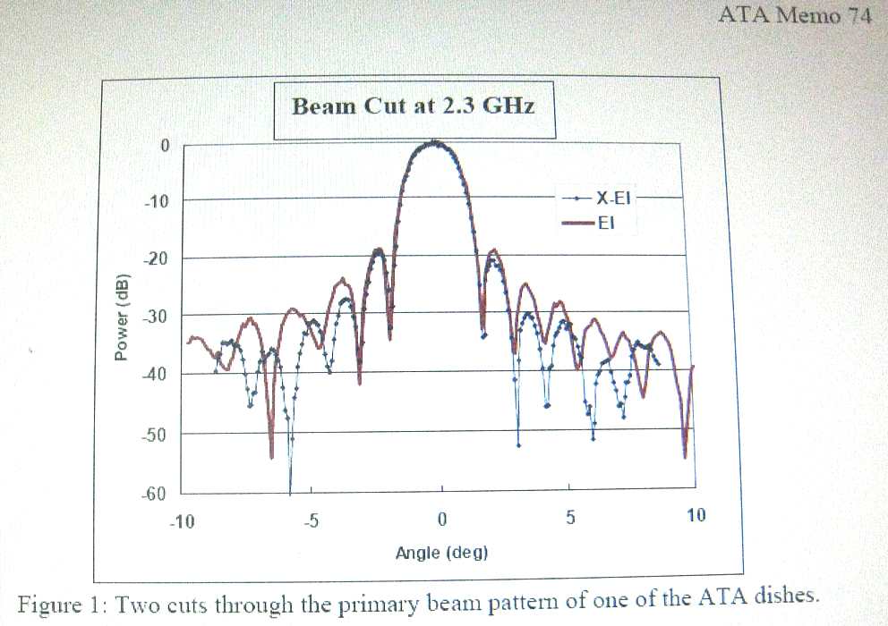
This is the measured main and side lob pattern of the ATA style antenna, as found in Memo #74. Simulations of Primary Beam Sidelobe Confusion with the ATA Primary Beam G. R. Harp and M.C.H. Wright, May 20, 2007" http://ral.berkeley.edu/ata/memos/index.html

Beam Forming Simulations
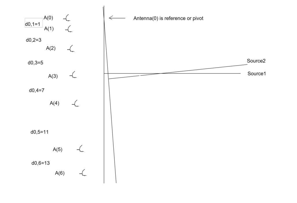
We have wave fronts arriving at all different times. Here is a 1-D representation of a line of antennas receiving a (flat) wave front from two sources. One perpendicular, wave front arrives at all antennas simultaneously. Two, off to one side, antennas receive the wave front at different times. The task is to later on to delay the signals from the different antennas to have the selected wave front appear to arrive concurrently. This will form a "beam".

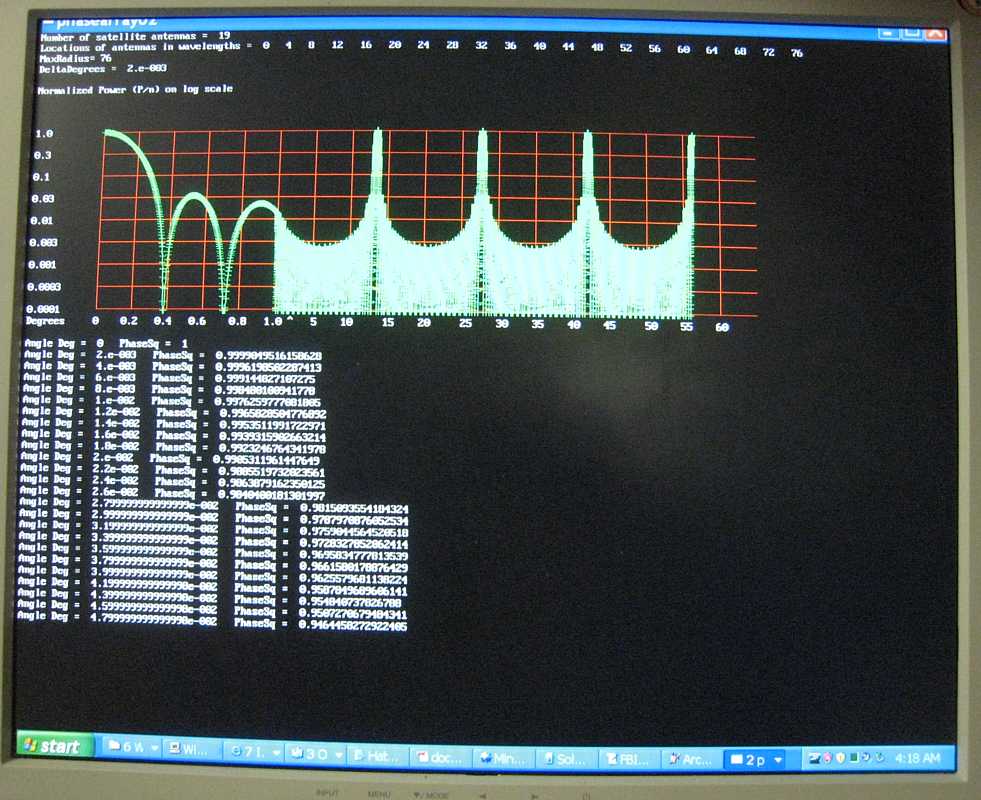
Here is a simulation of a straight line (1-D) array of 20 non-directional antennas separated by 4 wave lengths each. Note the rather narrow main lobe (3 dB down at 0.2 degrees) at zero degrees, and the major side lobes at 13. 27 and 57 degrees. In the case of ATA, the antennas are larger and can't be that close, but are directional and the major side lobes should be heavily suppressed (not received). The science and art (in 3 Dimensions) of antenna placement is "interresting".

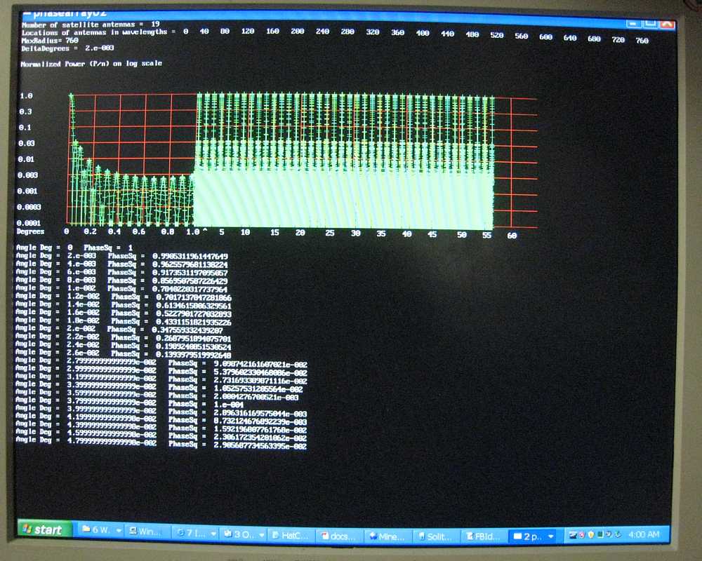
Here is a simulation of a straight line (1-D) array of 20 non-directional antennas separated by 40 wave lengths each. Note the narrower main lobe (3 dB down at 0.02 degrees) at zero degrees, and the horrible side lobes. The goal of the antenna farmers is to preserve a narrow beam with while suppressing side lobes.
If the strong side lobes were far away from the beam width of each individual antenna (say 5 degrees), the situation would be better - baring local interference - but clearly the orderly arrangement shown here seems useless.

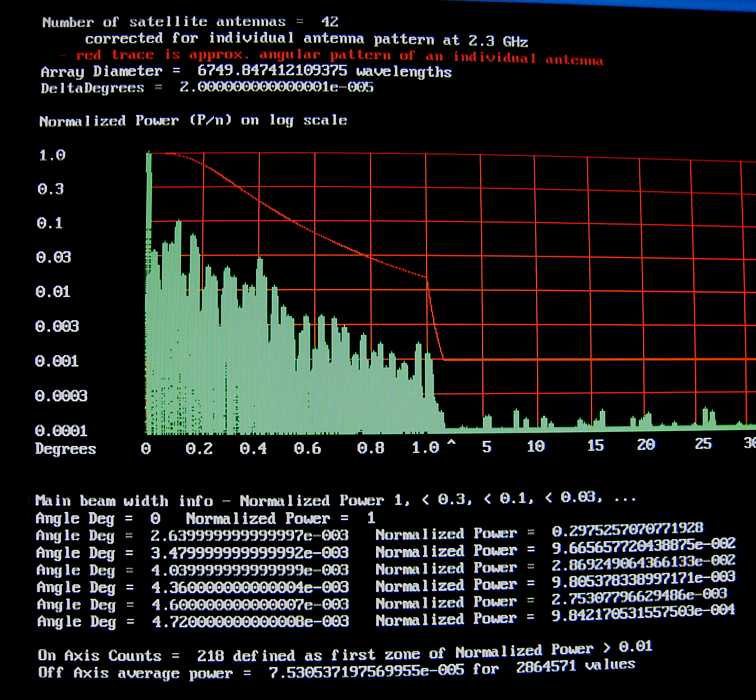
Here is a simulation of a straight line (1-D) array of 42 non-directional antennas in a random order 7,000 wavelength wide. I think ATA Phase 42 will approximate this at 1.4 gHz. The current layout seems about 100 meters?? diameter Note the narrow main lobe at zero degrees, 
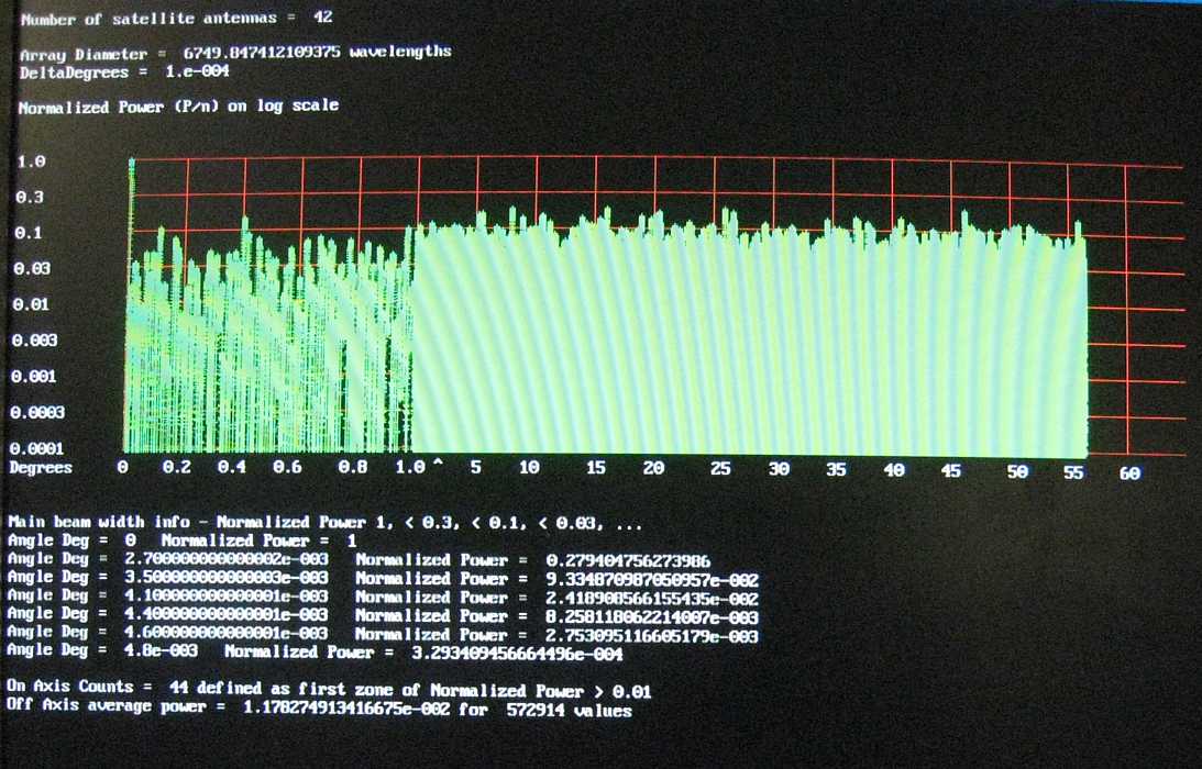
Right - is the simulation using the approximate pattern of the 20 foot individual antenna, the red trace.

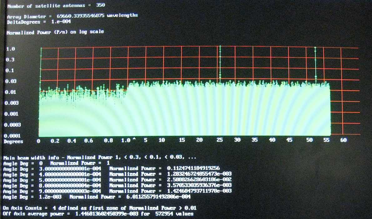
Here is a simulation of a straight line (1-D) array of 350 non-directional antennas in a random order 70,000 wavelength wide. Info indicates the ATA full site at 700 meters wide? I think ATA will approximate this at 1.4 gHz. Note the much narrower main lobe at zero degrees, and the side lobes near 27 and 53 degrees. Fortunately the individual antennas have a beam width of 5 degrees, and these side lobes should be extremely attenuated.
The average side lobe power (treated as noise) is 1.4 E-03 dB of the main lobe.

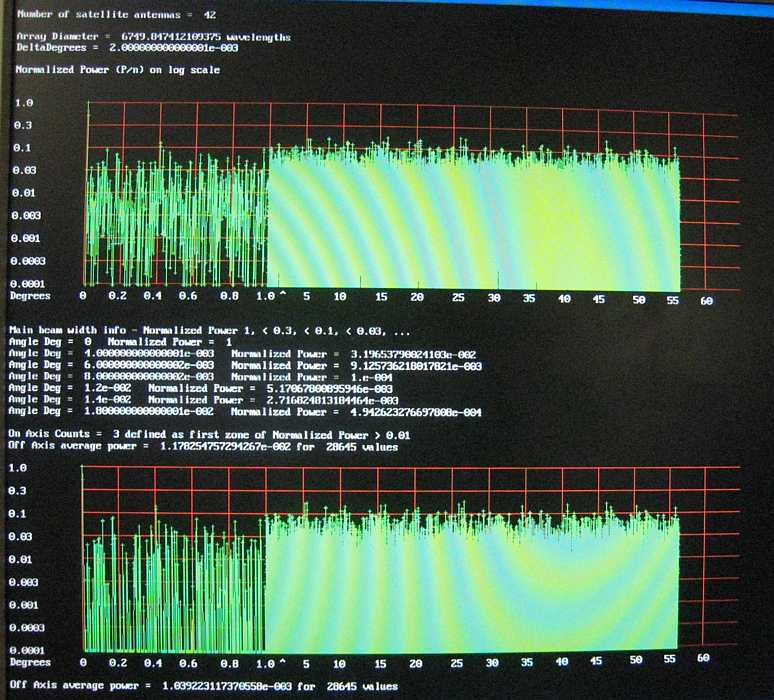
Back to the 42 random antennas. I wondered why people go to the trouble of running N*(N-1)/2 correlators when it seems less bother to run N phase summations with the same inputs. So this is phase summing on top and correlators on the bottom. it seems that the side lobes (treated as noise) is reduced by 10 db doing correlation - and I can't guess why.
- Phased side lobe average power = 1.17*10^-2 db
- Correlated side lobe average power = 1.04*10^-3 db

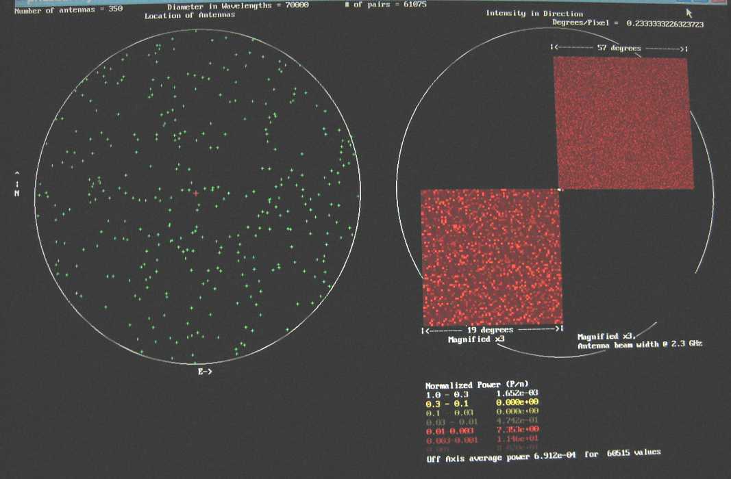
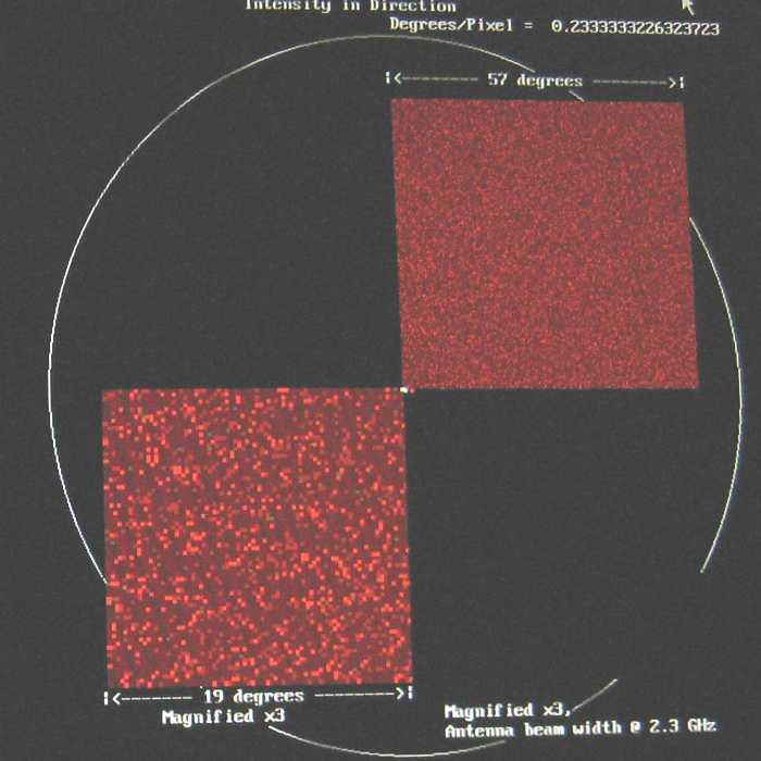
This is a 2D simulation of side lobe power of 350 randomly placed ATA antennas in a 70,000 wavelength diameter circle - no attempt at optimization. Focus is vertical, center white dot, Normalized power there is = 1.0. code. See this memo for a fuller view of the complexities involved.
  • Upper right - quarter field 1 radian, 57 degree wide, non-directional antennas
  • Lower left - magnification x 3, mirror image of upper right, non-directional antennas
  • Lower right - mag x3 flipped of upper right, corrected for antenna beam width, reducing side lobes about 25 db

The above simulated images of a random un-optimized field of ATA antennas might look optimistic. Looking at the lower right square which was approximately corrected for the beam width of an ATA antenna at 2.3 gigahertz seems visually good -
But there are very powerful noise sources, as pointed out in Memo #74 above. Our Sun, Cas A, Cyg A, are sufficiently powerful to require added work to get reasonably clean "images" when they are above the horizon.

Lets assume that the antenna farmers (the folks who decide where to place the antennas) do a much much better job -
But a computational optimization problem of enormous proportions.
I don't even know if they have a quality factor to judge numerically if one pattern is better than another :-((

The above simulations and discussion does not approach nulling of the array to reduce the effect of one or more serious serious RFI sources. Your attention is drawn to the "null steering" part of Customized Beam Forming at the Allen Telescope Array G. R. Harp, August 12, 2002

----------------------------------------------------

and computers and Trigonometry and Time

All over the place is Trigonometry - but you and I don't want to dive in very far. Just look at the changes with Time during the observation time.
  • Where is the star in the sky (the astronomers have a convention based upon the earth's revolution about the sun. Unfortunately the this is not constant, so actual sky maps refer to epochs - changed about every 50 years. Our beam widths are narrow enough that earth referenced positions stars must be updated "frequently".
  • The earth turns relative to the stars in a relatively constant manner every "24 hours". Actually the "24 hours" refers to an idealized sun position at "noon". Since the earth's orbit is not a circle, astronomers speak of "mean solar day".
  • But the sun appears to move in the sky relative to the stars, so the astronomers speak of siderial time - a sidereal day - 1 sidereal day = 23.9344696 hours (or: 23 hours, 56 minutes, 4.091 seconds).
  • So - finding and continuing to point a star is not so easy.
  • But there is more - using the altitude-azimuth (altazimuth) telescope mounts common (much lower cost) in astronomy now,
    • You must constantly change both the telescope's altitude and the telescope's azimuth. The telescope is not a sidereal clock on a polar mount like the good old (expensive) daze.
    • AND the stars in the view of a sensor (film, CCD, feedhorn) rotate in the field. In optical telescopes, you must rotate the film or other light sensor as time goes by, or the stars not at dead center will appear to rotate in a circle about the center of pointing - much as the Big Dipper appears to slowly rotate to people staring at it.
    • And the polarity of the light or radio waves also changes with the rotation.
  • And likely more things I forgot or haven't learned - all involving Trig & Time & changing Frames of Reference
  • SO - Dear Friends - aren't we glad we sell shoes (or what ever) rather than study this part of astronomy :-))

So, taking off the gloves,
  • For starters we will assume that our ATA array is in carefully arranged, carefullly surveyed fixed places on a flat plain at Hat Creek, north of the equator, west of London. (many corrections to be incorporated later)
  • Our particular target star is offset from the tracking point, one of several being examined concurrently by the various astronomers in the current field of view (lets say in a circle 10 moon widths diameter)
  • And of course we have a good regular clock adjustable to sidereal time and to run the radio equipment.
  • The "antennas" have been carefully leveled, the poles are streight up, the azimuth and elevation corrections carefully made, the antennas are uniform in construction, ...
  • The communications to the antenna drive servos and from the antenna receivers is fully functional (OK, a few antenna are listed out of service with problems, but that is the way of the world) ...
  • The above is enough to get us started on our wild ride into practical phased array radio astronomy. :-))

This is a diagram of the signal from the antenna(s) into the system.
The color codings are used below.
RF Conversion After the analog laser signal is received from the "front end" into the computer area, it is converted back into the original RF and hetrodyned into a frequency range for digitizing (analog to digital converter) using oscillators (not shown) and this RF Converter - the square red box. Note there are 4 local oscillator frequencies and 4 independent "base band" output from each Converter. I think there are 42 of these boxes, one per antenna.
to the right is a drawing from the picture
Beam Forming So we feed the Intermediate Frequency (Base Band 100 MegaHertz) (not rectified - still has phase info) into a ?800? million samples/second Analog to Digital converter and into a variable delay system - maybe like this memory based delay line where the read information is taken from areas written the correct number of "Desired Delay+1" clock pulses from where the data was written. Kind of a ring buffer with a variable length.
Beam Former Electronics - one of the green boxes. Each box can programmably delay four different phase pairs. I think there are 42 x 4 = 168 of these boxes.
from http://www.seti.org/ata/gallery07/ "Beam former electronics for the Allen Telescope Array"
and a drawn version of an individual module is to the right

Although Beam Former Electronics is relatively simple to implement at low clock frequencies, say 20 megahertz, operation of groups of these things at a clock rate of 40 times higher involves circuit delays due to the speed of light in a bleeding-edge-of-the-art way. There are a number of schemes to try to help but the experience would seem painful at best. Time synchronization must be a real bear - down to the nanosecond - You are sampling each 1.25 nanosecond - a nanosecond jitter or uncertainty is a high percent of your error budget.

Q & A with Gerry Harp

Beam Former - Visit to Berkeley Oct 22,2007 - to Geoff Bower GBower (at) astro.berkeley.edu & a seminar

Visit to Geoff Bower - I referred to my drawing (above) of a possible Delay Unit - suitable for Beam Forming (at much lower data rates - present FPGAs are too slow for the above configuration at 800 mHz, or even 80 mHz?)
Goeff said that this could likely work as I described, but the real thing has some added components -
  1. The same logic could delay both polarizations - (I forgot about polarization when making the diagram)
  2. Between the indicated ADC and Dual Ported Memory is a 200 mHz FIR digital filter
    (Goeff actually said something was "down converted" to 200 mHz - but that confused me. So I changed the words and meaning to the above.)
    Unfortunately, the above diagram seems unrelated to this approach - http://casper.berkeley.edu/papers/beamforming.pdf so maybe I'm barking up the wrong tree. (I plan a trip to ATA in a week to try to correct my understanding ;-)
    The trip was fun - but did not increase my understanding
    - now studying digital down converters and digital radios -
    http://www.mathworks.com/applications/dsp_comm/demos.html?file=/products/demos/shipping/filterdesign/ddcfilterchaindemo.html#1
    I guess I should have taken up digital filtering !!
    The CIC filter - http://beamdocs.fnal.gov/DocDB/0015/001529/001/The%20CIC%20filter.doc
    Does the quadrature output from a quadrature type mixer (or balanced detecter?) add information (about the phase of the local oscillator?) and is it useful?
  3. After the Dual Ported Memory is another filter that enables finer resolution phase shifting than offered by the 800 mHz sampling (1/8 wave at 8 gHz - maybe 1/6 wave at 11 gHz)
  4. Final channel gain (and some other?) corrections to the data stream are made after the Dual Ported Memory before being shipped out to the next device.
  5. There are modifications to permit present FPGAs to handle the high speed tasks. Future FPGAs are expected to be even faster.
Apparently both summing and correlation are used after the above delay unit
- summing as it is cheaper, easier
- correlating some pairs of antennas to get increased ?sensitivity? to actual relative delays, amplitudes, and ????

There are indeed four independent dual channel (for polarization data) per plug-in chassis (above).

I pressed for more details, and maybe drawings, but Geoff suggested that I really go to the site to get more details.

-----------------------------------
I hope I got some of the above correct -

Geoff was between meetings, and very kind to talk with this drop-in
and I was slightly late for the seminar I had come to see.

comments on the above section by Matt Dexter - Sept 2008

Regarding
  http://ed-thelen.org/ATA/HatCreekATA-StrugglingOn.html#BerkeleyOct22
Our current FPGAs could not fit the interpolating filters to get
to delay steps finer than the 838.8608MHz sample clock resolution.
Just not enough gates. 1/838.8608MHz is as fine of delay step
as is supported at the moment.

At this time only the FPGAs programmed for the Transient Search, aka Fly's
Eye, experiment have fine channel gain correction on the 8bit I + 8bit Q
voltage samples just after the digital down conversion. The FX correlator
has gain correction on the F engine's output 1024 spectral channels which
are 4bit I + 4bit Q voltage samples.


There are two usual ways to collect data from objects using radio telescopes:
  1. Point the radio telescope, dish or phased array, and use the rotation of the earth to bring the desired object through the fixed beam, recording the data (amplitude, frequency, phase, ...) versus time, and map that portion of the sky using the recorded variable(s) and time. This method is less stressful on the pointing mechanism (if any).
    The earth rotates at about 15 degrees/hour relative to the sun, or about 0.25 degrees per minute. (Slightly less if observing stellar objects (sidereal rate). The approximate beam width for ATA at 11MHz is wavelength/diameter or 0.025/700 meters or 3.6^-5 radians or 0.002 degrees. With the earth rotating at 0.004 degrees/sec, a point source would be in the beam width about 2 seconds. This may be great for mapping strong sources, but not great for other sources.

  2. Actively point the dish or phased array at the desired object for an extended time counteracting the rotation of the earth. This method permits longer observation (or integration) time for weak sources. This method is identical to optical telescopes. The telescope must move at a precisely controlled rate. If the telescope mount is not "polar" the image rotates and this rotation must be corrected for.

Lets put in some numbers for a phased array about the size and frequency of the Allen Telescope Array - lets assume a maximum diameter of 700 meters, a radius of 350 meters. 350 meters times sin(0.25 degrees) = 1.53 meters per minute or 0.0255 meters/second or about 2.55 centimeters/second. This is about one 11 MHz wavelength per second (the top ATA frequency).

To allow a wide pointing angle (approaching 90 degrees), we should allow for delay times of plus/minus 350 meters. This is about 14,000 wavelengths a 11 MHz. To reduce noise and errors caused by delay units, probably we should allow at least 10 delay increments per wave length. The delay counters should be plus/minus almost 320,000 counts. A count of 2^20 can represent over 1,000,000 counts.

In a previous paragraph we showed that there is about 1 wavelength shift per second at 11MHz. To allow 1/10 wave length error, the delay unit must be updated about 10 times per second max. This starts to stress conventional updates from a normal computer - so additional help must be applied to obtain adequate synchronization of delay data updates. This can be achieved by allowing the computer to update buffers and controls on say a ten second basis, then the clock system can send a sync pulse to update all delay controls simultaneously. The computer obviously needs access to a good (sidereal) clock.


Collection of stuff
some time stuff
- a sidereal second is shorter than a solar second
- epoch - due to earth's polar precession
Collection of words
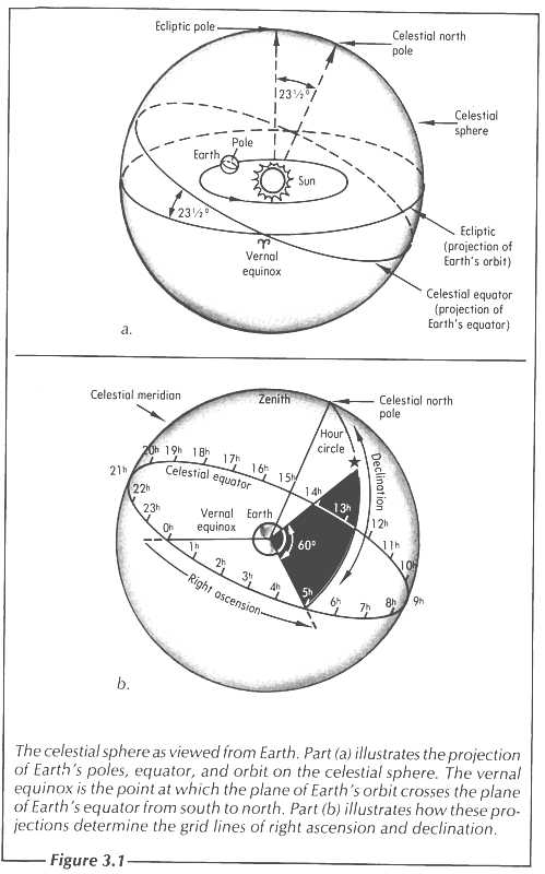
some declination stuff - latitude
  • celestial equator is a great circle on the imaginary celestial sphere, in the same plane as the Earth's equator. In other words, it is a projection of the terrestrial equator out into space. As result of the Earth's axial tilt, the celestial equator is inclined by ~23.5° with respect to the ecliptic plane.
  • astronomical latitude, This is the angle between a plumb line and the equatorial plane. Although [Schrieber 1943] implies that Geodetic latitude is Astronomical latitude, there may be up to a minute of arc difference between the two [Bowditch 1958].
  • Geodetic latitude. This is the angle between the normal to the surface of the ellipsoid and the equatorial plane. This variety is also called Geographic latitude and is used on maps. However it is a right pain to calculate with, but came into use because it is closer to the astronomical latitude which people can measure with a sextant. I will denote it by small case t.
  • Geocentric latitude. The angle between a line joining the point on the surface of the earth and the center of the earth, and the equatorial plane. I will denote it be t and use it in most of the subsequent calculations.
  • Geographical latitude, which is used in mapping, is based on the supposition that the earth is an elliptic spheroid of known compression, and is the angle which the normal to this spheroid makes with the equator. It differs from the astronomical latitude only in being corrected for local deviation of the plumb-line.
    http://www.1911encyclopedia.org/Latitude
Variability of Terrestrial Latitudes http://www.1911encyclopedia.org/Latitude
Collection of words
some ascension stuff
  • right ascension (small greek alpha?a) -also RA-, or hour angle (H) -also HA-
  • IBOB is "Internet BreakOut Board" capable of using XAUI protocol - has a Power PC to be programmed
  • CICADA - Configurable Instrument Collaboration for Agile Data Acquisition (CICADA) nrao
  • CASPER - nrao green bank
  • ADC - in line with IBOB - modes = interleave and not interleave
  • BEE2

Pointing the array