Go Forward, Go Back, Go to Table of Contents, Go to On Line Documents, Go to Go to Antique Computer home page


Reckoners, ENIAC, page 0104


5
Faster, Faster: The ENIAC


.
In 1746. . .I met a Dr. Spence, who was lately arrived from Scotland, and who show'd me some electric experiments. They were imperfectly perform'd, as he was not very expert, but being on a subject quite new to me, they equally surpris'd and pleased me. Soon after my return to Philadelphia, our library company receiv'd from Mr. P. Collinson, Fellow of the Royal Society of London, a present of a glass tube, with some account of the use of it in making such experiments.
-Benjamin Franklin, Autobiography

People often speak of computers as belonging to one of several "generations" beginning not with the machines discussed in this book but rather with the first commercial computers. That term implies a linear evolution of machines and technology. But it is a misleading analogy: the computer did not descend from one or two ancestors. The first ones incorporated bits and pieces from this and that machine: punched tape from telegraphs, relays from telephones, punched cards from accounting machines, vacuum tubes from radios. And so it goes today. Living creatures do not evolve that way. (Mythical creatures like the Centaur combined the best qualities of the man and the horse; but among living animals maybe only the Missouri mule is close to illustrating how machines evolve.)

But if there is a "granddaddy" of all the generations of digital computers, it would have to be the ENIAC, the first working electronic numeric digital computer. It was not a "first generation" computer, since it was not used commercially. Perhaps it belongs to the "zero" generation, since nearly every computer built thereafter owes something to it. What they owe is the subject of this chapter.


Reckoners, ENIAC, page 0105

The ENIAC was an electronic computer: it was the only early computer except for the British Colossus that computed at electronic speeds. But like all the machines of its day it was a transitional device. It had some relay circuits. It was programmed like an IBM accounting machine. It was a computer, a powerful and fast computer at that, but its design and programming did not become the basis for any computers thereafter. Nothing quite like it was ever built again. Like the Harvard Mark 1, the most important thing about the ENIAC was that it existed: it proved to the world that computing at electronic speeds was indeed possible, just as Howard Aiken had proved that Babbage's dream was more than just a dream. In 1945, when the ENIAC ran its first programs, that was important.

What is so important about computing at electronic speeds? The ENIAC computed about 500 times faster than any of the electromechanical computers, a difference of scale that made it an entirely different type of machine. With a relay machine it was always possible to measure computing power in terms of the number of human beings it could replace-that was the measure used in the published accounts of the Bell Labs machines and the Mark 1. But the ENIAC was built precisely to tackle a job that by nature was beyond the capabilities of human-or electromechanical-computers.

That was not the first time the pace of technology outran its conceptual understanding. The first steam engines were measured by their "horsepower" -how many horses they could replace for a given task. Matthew Boulton and James Watt charged for their machines accordingly. But a modern diesel locomotive, developing hundreds ofhorsepower, could never be replaced by an equivalent number of horses. (The problem is not getting all those horses hitched together; it is getting them all to pull in the same direction: to coordinate each horse's power in a meaningful way.) The same is true regarding the ENIAC: it broke through the limits of human computing power, power limited by the fact that if a computing team was too large, its work could not effectively be coordinated. (Incidentally, although little information about the British Colossus has been made public, it is clear that its designers also recognized the absolute importance of electronic speeds for the job of breaking the German codes the British had intercepted. No electromechanical machine could have done it.)1

By 1943 Helmut Schreyer in Germany and engineers at IBM and RCA had designed electronic calculating circuits. National Cash Register was looking into the possibility of using vacuum tubes in its machines. There were no doubt many other examples from that time which have not yet come to light; using electronic circuits for all-or-nothing switching was fast becoming an accepted idea.2

In the late 1930's, Professor John V. Atanasoff of the physics department of Iowa State College (now Iowa State University) conceived of the idea of using vacuum tube computing circuits to solve systems of linear equations. He got pretty far with that idea-farther than Schreyer, to be sure-but the machine was stalled in its final stage of construction and never did any useful work. Around the same time, at Ursinus College in Collegeville, Pennsylvania (near Philadelphia), Professor John Mauchly was also thinking about computing with electronic elements. He built a few test circuits, and after meeting Atanasoff in 1940 at a meeting of the American Association for the Advancement of Science, he stepped up his efforts to build a digital computer.


Reckoners, ENIAC, page 0106

Mauchly moved from Ursinus to the Moore School of Electrical Engineering (part of the University of Pennsylvania), at first to learn more about electronics, then staying on as an instructor. There he teamed up with J. Presper Eckert, who had been one of his instructors. From that point the story is not clear, but it seems that Atanasoff's machine was the spark-a small one, but a spark nonethelessthat ignited Mauchly's enthusiasm about electronic digital computers. He and Eckert transformed that enthusiasm into a working computer: the ENIAC. And from the ENIAC came almost everything else.3

Well, not quite. That progression from Atanasoff to the ENIAC to the modern computer is not untrue, but the story is hardly so neat and tidy as it implies. An elaborate genealogical chart of the evolution of the computer, full of begettings like the Book of Genesis, obscures the tortuous paths that were really taken.

The question of just who really invented the ENIAC (and by implication, who invented the electronic computer) is fraught with controversy; it has even been the subject of a lawsuit. (The lawsuit has been settled, but the controversy remains.) But there is no doubt as to why the ENIAC was invented: it was designed for one specific wartime problem: the preparation and printing of firing tables. Had there not been such a need for those tables, the ENIAC would not have been built. Eventually of course someone would have built an electronic digital computer, but it would not have been the ENIAC,4 (Computer designers today often do not care about what their creations are used for; they build a machine that can execute certain general "benchmark" programs that test the machine's overall abilities. But that was certainly not true in the 1940's.)

FIRING TABLES

The heavy artillery used in World War Two had remarkable range: some guns could fire a shell twenty miles and more. But that range was useless if the shell could not hit its target. At short ranges the gunner can see the target and make adjustments on the spot; at longer ranges he can station a forward observer to radio back some of that information. But even in those cases he needs a firing table: a table of numbers telling him how to set the firing angle to give him the range he needs. A firing table is simply a table of angle settings and the corresponding ranges they give for a given piece of artillery. The table also gives the velocity of the projectile at impact (needed if it is to pierce an armored target) and perhaps also the angle of fall at impact (needed if the projectile is to clear a rampart or other obstruction).5

An analysis of the trajectory of a shell quickly leads to higher-order differential equations, as is so common in describing physical phenomena. The basic physical law is of course Isaac Newton's: an object in the earth's gravitational field falls with a constant acceleration. Acceleration is the rate of change in the velocity of an object; the velocity is the rate of change of the object's position. To find the position of a shell at the end of its trajectory thus requires the solution of a second-order differential equation; to find its terminal velocity requires solving a first-order equation.

That relationship is only a starting point for the preparation of a firing table. The most important additional factor is the resistance of the air. It in turn varies according to the temperature, humidity, and altitude through which the projectile travels; it also varies according to the shape of the projectile. But in the main the air resistance is a function of the velocity of the projectile: the greater the velocity the greater the resistance. So an analysis of the air resistance also leads to a differential equation.

The gunnery officer in the field could not be expected to do the math required to compute a trajectory. Instead he consulted a table for the type of gun and shell he was using. That table could not be so complicated as to be unreadable under battle conditions. Firing tables usually listed just the range and velocity for a given firing angle, with supplemental tables of correction factors for things like crosswinds, other weather conditions, even for drift caused by the rotation of the earth.

What all that meant was that a lot of computation was required for the preparation of even one firing table, and for the many types of guns and projectiles being developed for the war, a lot of tables were needed. The differential equations derived for a trajectory were of the type that could only be solved numerically: that is, it was not possible to find analytic solutions that yielded the trajectory of the shell directly. As with the equations faced by Howard Aiken, trajectories were computed by combinations of elementary operations of arithmetic together with temporary storage of intermediate results and the consulting of tables of mathematical data.6 The computations were long, tedious, and prone to error, even when done with the aid of desk calculators.

In the 1930's, Vannevar Bush had built an analog computer that could solve differential equations, using a mechanical integrator similar to the familiar device that computes a household electric bill. The basic computing element of his "Differential Analyzer" was a rotating disk, upon which rested another smaller disk whose rotation corresponded to the integral of the desired function. (The watt-hour meter measures the integral of the power a household consumes with respect to time. The power is the product of the voltage, which is a constant 110 volts in America, times the current, which varies from moment to moment depending on what electrical appliances the customer is using. The meter performs that integration by translating those functions into analogous motions of the rotating disk, thereby computing the kilowatt-hours for which the customer is charged. Bush's Differential Analyzer used a more primitive mechanical version of that disk integrator.)7

It was an enormously complex machine. By 1942 Bush's Analyzer had been rebuilt and fitted with a number of improvements that gave it more speed and power. Eventually its size and cost put it on a par with the first digital computers such as the Harvard Mark I, although it worked on entirely different principles.


Reckoners, ENIAC, page 0108

The Differential Analyzer was faster than teams of human computers using desk calculators, but it was still not fast enough. The Moore School of Electrical Engineering at the University of Pennsylvania built a copy of one, and used both it and human computers (mostly recent graduates from women's colleges up and down the Eastern Seaboard) to compute trajectories. Humans took at least several hours to compute a trajectory. The Differential Analyzer could compute one in about twenty minutes. But it was a complicated, unique piece of machinery, and setting it up to compute a specific trajectory took time, during which the machine could do no work. By mid-1942 Ballistic Research Laboratory (BRL) officers realized that neither method could keep up with the ever-increasing demand for firing tables.

So it was against that background in 1942 that John W. Mauchly of the Moore School wrote a memorandum entitled "The Use of Vacuum Tube Devices for Calculating," in which he proposed that an electronic computing device be built to solve differential equations, not by the analog method of the Differential Analyzer, but by the numerical methods used by the teams of human beings with their desk calculators. The difference would be that electronic, not mechanical, devices would perform those calculations, and electronic circuits would furthermore coordinate the elementary arithmetic operations and transfer and store intermediate results automatically. With that approach, Mauchly said, the time needed to compute a trajectory would drop to a minute or two.8

In April, 1943, that memorandum grew into a formal proposal by Mauchly, J. Presper Eckert, and John Grist Brainerd for a machine which would retain the automatic operation of the Differential Analyzer, yet use the numerical method that humans used, and do the job much faster than both. They called the machine an "Electronic Diff.* Analyzer," with a footnote referring to the abbreviation "Diff." as meaning not "differential" a la Bush's analog computer, but rather "difference," as in the use of finite differences manipulated by ordinary arithmetic. (The term "digital" had not yet come into common use, but that is clearly what they meant.) Soon after the project received funding, Colonel Paul Gillon of the BRL gave it the name ENIAC, for "Electronic Numerical Integrator and Computer."9

The idea of building the digital electronic computer was Mauchly's. He was an instructor at the Moore School, but his primary interest was not electronics but meteorology. From 1933 to 1940, while he taught physics at Ursinus College (he was a one-man physics department), he recognized the need to automate the process of computation to advance the art of weather prediction. Weather prediction was at that time just getting a theoretical foundation that showed great promise. Led by Lewis F. Richardson in England, meteorologists had developed sets of equations that, while only a crude approximation of the immensely complex patterns of the weather, nevertheless offered a chance of making reasonably accurate predictions. But their advances required large numbers of computations, and their work was held up in the 1930s's by a lack of computing power.10


Reckoners, ENIAC, page 0109

Mauchly explored the familiar computing techniques of his day: mechanical calculators, punched card equipment, and electronic circuits, both digital and analog. To learn more about electronics he enrolled in a special course at the Moore School designed to acquaint people with that fast-developing technology, and ended up staying on. J. Presper Eckert was a graduate student at the Moore School who was an instructor in that course. He had been working on various war-related projects, including work on the copy of the Differential Analyzer the Moore School had. Eckert had helped convert some of the machine's units from mechanical to electronic operation, but other than that he had not done much work in computing. But Mauchly's enthusiasm was enough to convince him; his facility with electronics was the perfect complement to Mauchly's vision of high-speed computing machinery.

In December, 1940, Mauchly met John V. Atanasoff and learned that the physics professor from Iowa State had already gone a long way toward building an electronic digital computer. Atanasoff was building a machine that could solve systems of simultaneous linear equations-the same sort of problem that Konrad Zuse was tackling in Germany. But Atanasoff had proposed doing it with electronic circuits, not relays. What was more, Atanasoff had quickly seen the advantages of a digital machine-that is, one that would solve those equations by numerical processes, not by representing the quantities by electrical analogs of voltage or current levels. Other physicists had developed special-purpose machines that could solve systems of linear equations. But Atanasoff's was far more advanced than any of them, both by his use of high-speed electronic circuits, and by his adoption of digital methods of solution.11 By the time Mauchly learned of Atanasoff's project, a prototype model had been completed and was almost completely functional. It could handle equations having up to thirty variables, and performed arithmetic on all the variables in an equation simultaneously (reminiscent of punched-card methods). The machine represented numbers in the binary system, with a word length of fifty binary digits, corresponding to about fifteen decimal digits. It did not use floating point. Atanasoff has said recently that he had known of the binary system ever since grade school; in any case, he chose the binary scale for his machine after carefully considering several number bases from the standpoint of maximum theoretical efficiency.

The only part of the machine not working was the input/output device, which was to have coded and read binary digits on cards at very high speed, much faster than commercial punched-card machines could. Mauchly saw that prototype on a visit to Ames, Iowa, in 1940, after meeting Atanasoff in Philadelphia.

Did John V. Atanasoff invent the electronic digital computer? That was the decision of Judge Earl Larson, whose 1974 judgement in a suit against Sperry Univac Corporation declared Eckert and Mauchly's ENIAC patent (which Sperry Univac had acquired) invalid for just that reason.12


Reckoners, ENIAC, page 0110

Atanasoff's machine had two features absolutely central to any modern conception of a computer: high-speed digital electronic circuits, and the binary system. We have already seen why electronic speeds are important. And while it is certainly possible to build a computer using the base ten (or any other base, for that matter), the advantages of the binary scale are overwhelming, especially so at electronic speeds. (The binary system is central to modern computer science; for freshmen computer science students binary arithmetic is the first thing they learn: it is the portal through which all must pass.) Konrad Zuse certainly recognized the practical advantages of the binary system. Atanasoff chose it after proving that it was the best system in theory as well.

Mauchly examined Atanasoff's machine carefully during his visit to Ames, and from his correspondence with the Iowa physics professor there is little doubt that he was impressed by what he saw. Mauchly was thinking about building an electronic computer, but it was only after seeing Atanasoff's machine (and after collaborating with Eckert) that his ideas crystallized into a practical proposal.

The ENIAC grew out of the proposal for an electronic "difference" analyzer. It was a digital machine, and it computed with electronic circuits. It did not use the binary system but rather used electronic versions of the familiar decimal wheels of punched card equipment. In that last regard it was far behind Atanasoff's concept (and Zuse's, and Schreyer's).

But unlike Atanasoff's machine, the ENIAC was programmable. It could compute firing tables, as it was designed to do, but it could also do a lot more-including solving systems of linear equations. Atanasoff stressed the fact that many problems of physics could be cast in the form of systems of simultaneous linear equations, and thus be solved with his machine, but there was no way that he could alter the sequence of operations that it went through. If in fact Mauchly derived his ideas for the ENIAC from Atanasoff, as Judge Earl Larson concluded, then he took an important step forward in proposing a machine whose sequence of operations could be altered by plugboards. But at the same time he and Eckert took a step backward in rejecting Atanasoff's decision to use the binary system.

But there is one final aspect to the story that clinches the argument. The ENIAC worked. Atanasoff's computer was never reliable enough to be put into routine use solving practical problems. If Howard Aiken's Mark I put Babbage's ghost to rest, then the ENIAC, which not only worked but worked well, silenced the many skeptics who said that no computer using vacuum tubes could ever be made to work reliably. Atanasoff's computer, had it been better publicized at the time, might only have added fuel to the skeptics' arguments. And in the 1940's, those arguments were taken very seriously. Charles Babbage first conceived of the idea of an automatic digital computer. John V. Atanasoff, together with Helmut Schreyer and perhaps others, first conceived of an electronic digital computer. John Mauchly and J. Presper Eckert, as leaders of a skilled team at the Moore School, invented the first working electronic numeric digital computer.


Reckoners, ENIAC, page 0111

BUILDING THE ENIAC

On April 9, 1943, Mauchly, Eckert (whose twenty-fourth birthday it was), and John Grist Brainerd submitted their proposal to the Army; it was approved not long afterward. Their first priority was to design the machine's accumulators the devices that would both add and store numbers like those in the Harvard Mark I, only at electronic speeds. They had to be designed before any other parts of the computer. Eckert was already familiar with high-speed electronic counting circuits, which by the 1940's were coming into wide use for counting cosmic rays and nuclear particles emitted from radioactive materials. In both cases the counter must run fast enough to keep up with the events it is counting. At the same time, because they counted large aggregates of events, accuracy was not too critical: it did not matter if they missed a particle now and then. (Absolute accuracy is generally not required in counters. Who cares if an automobile odometer is off by a mile or two?)

Most of the discussion about electronic counting circuits appeared in experimental physics journals, which discussed counting cosmic rays or other nuclear events. (Mauchly especially remembered many articles on counting devices that appeared between 1935 and 1941 in the Review of Scientific Instruments.) Those counters either used a gas-filled vacuum tube called a thyratron or else they were descendants of the so-called Eccles- Jordan "flip-flop," first published in 1919. That circuit contained a pair of "triodes"-three-element vacuum tubes-only one of which conducted current at any one time. When the circuit was triggered by an external pulse of current, each tube in it "flipped" into its opposite state: conducting or nonconducting. (H. J. Reich of the University of Illinois called the Eccles-Jordan circuit a "trigger" circuit in his writings, which were widely read. The IBM engineers working on electronic calculators in the 1940's remember the circuit by Reich's name; after the war the term flip-flop came into common use.)13

The flip-flop was thus fundamentally a binary device, but it worked on different principles from the bi-stable circuit that Helmut Schreyer developed for his doctoral thesis. Schreyer's device used a neon lamp instead of two triodes to maintain the state of the circuit. The Eccles-Jordan device was considerably faster. (Incidentally, Mauchly also investigated neon tube circuits while he was at Ursinus.)

The problem became one of choosing a counting circuit, of which there were plenty of examples described in the technical literature, and making it absolutely reliable. Remember that in a digital computer the loss of even one digit can spoil the results of a computation.14 The counters then in existence used a variety of number bases. Some counted cosmic rays in the binary system; others used rings of tubes that counted decimally by groups of four binary flip-flops, like George Stibitz's binary-coded-decimal circuits in the Complex Number Computer. Other counters used the bi-quinary system, like the later Bell Labs relay computers, using a total of seven tubes to count a decimal digit.


Reckoners, ENIAC, page 0112

The circuit Eckert and Mauchly chose for the ENIAC's accumulators coded a decimal number by ten flip-flops, one for each decimal digit. So it took twenty triodes to represent a single decimal number. Those ten flip-flops formed a ring that recorded a number just like the engraved wheels of a mechanical adding machine did. An adding machine's wheel indicated a number by whatever digit was visible through a window. The ENIAC's ring counters indicated their digits by whichever of the ten flip-flops had a different state than the other nine. When a pulse was sent to the ring, it turned off that flip-flop and turned on the one next to it. And when the ring received a series of pulses, they triggered a succession of flip-flops corresponding to an addition of that number. If, say, the fifth flip-flop was "on," and the ring received a train of three pulses, the ring would move from state 5 to states 6 and 7, and finally come to rest with the eighth flip-flop on, representing the sum of five and three. If a train of pulses passed through the nine's position, a carry pulse would be sent to the neighboring ring counter as well.15 The ENIAC's ring counter worked like the accumulators of Howard Aiken's Mark I, using tubes instead of wheels. (Eckert and Mauchly knew of the Bell Labs computers but not of the Mark I when they began designing the ENIAC.)

Writing a few years after the machine's completion, Eckert said that he rejected the binary and binary-coded-decimal systems because he felt they could not be made reliable enough.16 The biquinary code was rejected because "it required stable resistors, which were then much more expensive than they are now." More recently, he and Mauchly have given other reasons.17 The price they paid for their code was that to count a decimal number required many more tubes than, say, Atanasoff's or Schreyer's circuits needed. No other electronic computer after the ENIAC used that coding scheme. Many have represented numbers in base ten, but they usually have used a binary-coded-decimal circuit that requires far fewer flip-flops.

A bank of ten such ring counters (called decade counters) could store and add ten-digit decimal numbers. They were called, appropriately, accumulators, and they formed the backbone of the computer. Like the Harvard Mark 1, the ENIAC's arithmetic was distributed throughout the machine: the accumulators did the addition and subtraction; a separate unit did multiplication, division, and extraction of square roots.

The 1943 proposal called for a machine with ten accumulators, but once preliminary work showed the design was feasible, the BRL asked for a machine with twenty. Each accumulator could store and add ten-digit numbers plus their signs. They were mounted in a series of panels arranged in a long U-shaped configuration which, together with the other parts of the machine, filled a large room (Figures 5.1, 5.2).
Reckoners, ENIAC, page 0113

In the accumulators, the two triodes of each flip-flop were enclosed in the single tube 6SN7, so there were at least ten such tubes for each ring, 100 for an accumulator. Besides those, there were others needed to ensure that the ring functioned correctly. In fact, each accumulator had 550 tubes, for a total of 550 x 20 or 11,000 tubes for the accumulators alone. The original plans called for the ENIAC to contain 5,000 tubes; as finished it had over 18,000.18 Recall that in Germany at that time Helmut Schreyer was proposing a computer that would use about 2,000 tubes, a proposal rejected as being too ambitious. The British Colossus, the electronic code-breaking computer completed in 1943, also had 2,000 tubes. By the end of the war ten versions of the Colossus had been built. The ENIAC was by far the most complex piece of electronic equipment built up to that time. Probably no other machine with that many tubes in it has ever been built since, or ever will be built, either. Nowadays all that computing is done with solid-state flip-flops crammed onto chips the size of a fingernail. Tubes still have their place, but not in computers. The circuits of the ENIAC appear more


Reckoners, ENIAC, page 0114


Reckoners, ENIAC, page 0115

Figure 5.2. One of the ENIAC's Accumulators

and more arcane with the passage of years, although its logical structure can still be deciphered with little difficulty.
Reckoners, ENIAC, page 0116

STRUCTURE OF THE ENIAC

Besides the twenty accumulators, the ENIAC had a cycling unit, programming units, constant transmitters for the values of functions like the drag function of a projectile, and input/output facilities. In one respect the ENIAC was very different from any of the electromechanical computers. Its program, the sequence of elementary instructions that it was to carry out, was not supplied by punched cards or tape or filmstrip. The reason is clear: the ENIAC's circuits did arithmetic at electronic speeds. That speed would be wasted if the machine had to wait for instructions that were being supplied at mechanical speeds. If a paper tape supplied its programs or function data, as in the Mark I, the ENIAC's accumulators would spend a lot of their time idly waiting to be told what to do next. (The only other electronic computer from that era, the British Colossus, did use paper tape for the input of alphabetic data. Those tapes were mounted on specially designed transport mechanisms that moved with incredible speed. Accounts of the Colossus in action describe tapes flying through the machine, feeding in up to five thousand characters per second. The tape itself quickly wore grooves in the steel guide pins, and since no take-up reel could handle that kind of speed, the tape simply was allowed to pile up at the side of the machine, describing eerie rainbow arcs in the air before settling to the ground in a heap.)19

So the ENIAC's instructions were wired into the machine by cables that connected its various parts to one another. Programs were changed by plugging in the cables in a different configuration. I shall have more to say on its programming later.

The ENIAC was a synchronous machine: that is, a central clock coordinated all its actions. Times for all elementary operations were precisely specified as a number of pulses sent out by the cycling unit. At each basic cycle, the cycling unit sent out a set of pulses, each of which had a specific role in controlling the computer. All numbers, algebraic signs, instructions, etc., originated as combinations of pulses from the cycling unit. That is, if the number 5 was to be sent from one accumulator to another, the first accumulator would not transmit five pulses to the other one, but it would rather open a "gate" at the second accumulator long enough for five pulses originating at the cycling unit to be passed through. The reason is that pulses lose their shape and intensity quickly. If a pulse that originated at one accumulator traveled through various other parts of the machine, it would soon be so weak that it could not do its job. Therefore all information in the ENIAC was transferred by sets of pulses freshly generated 5,000 times a second by the cycling unit. Even with that arrangement, the accumulators also had "pulse-reshaping" circuits that restored the strength of signals as they arrived.

The basic cycle was 200 microseconds, one addition time. During a cycle ten parallel pulse trains went out. Each had a specific role in controlling the machine. The first, for example, consisted of one pulse 2 microseconds long that came near the end of the 200 microsecond cycle. Its job was to advance the programming units of the computer to their next program step, as specified by the setting of program switches and the plugging of program cables. The second of the ten trains consisted of ten 2-microsecond pulses that came at the beginning of the cycle. Its job was to cycle a ring counter whenever a number was to be read. In this way the contents of an accumulator could be read out by cycling the counters one full revolution, after which each would have returned to its original position.


Reckoners, ENIAC, page 0117

The next eight trains had similar roles. All but one of them consisted of strings of pulses that were 2 microseconds long, separated from each other by a space of 8 microseconds. Thus the shortest sub-cycle of the ENIAC was 10 microseconds, or a clock frequency of 100 khz (that is, 100,000 cycles per second). For diagnostic purposes it was possible to slow the machine down so that it executed just one of those pulses at a time, or one full addition cycle (twenty pulses long) at a time.

One of the pulses, the "carry-clear" pulse, was 70 microseconds instead of 2 microseconds long, as were the other nine. The reason for that was that during an addition, all ten digits of a number were transmitted simultaneously. Should one of those transfers cause a carry of ten to the next ring counter, that carry had to be held until the next counter was finished with its addition; otherwise it would be receiving two pulses at once and would not know how to sort them out. Recall that the ten-pulse mentioned above came at the beginning of an addition cycle. Once all the digit pulses were sent, the carry-clear pulse opened up a gate and held it open long enough for any carries to take place. In the extreme case where a carry propagated itself through all ten decimal places (for example, 1 + 9,999,999,999), that could take up to 25 microseconds, as determined by experiment. So the carry-clear pulse held the gate open long enough to make sure that all the carries got through. An addition therefore took ten short pulse-times to cycle the ring counters, one 70-microsecond pulse-time for the carries, and three short pulse-times for complementing, resetting, and control, for a total of 200 microseconds that made one addition cycle (Figure 5.3). The ENIAC could add 5,000 numbers per second.20

A computation proceeded by gating appropriate pulses from the cycling unit around the various arithmetic units of the machine, ending at an accumulator connected to a printer or other output device. So the basic flow was clockwise around the U-shaped configuration, but for all but the most trivial problems there would be multiple paths of number-routing, looping of operations, and branching back to a previous sequence of operations. All that was controlled by the programming units, described next.

The solution of, say, a differential equation implied a combination of elementary arithmetic operations, storage and retrieval of intermediate results, and consulting tables of functions or other data. Machines like the Z3 supplied those operations in a linear sequence, coded into perforated film that passed through a reading device. The ENIAC's program was supplied by rewiring the machine for each specific problem, then directing a programming unit to step through those operations in the proper order.


Reckoners, ENIAC, page 0118

One implication of that scheme is that there is no reason why the steps have to be executed one at a time in a sequence. The programming unit could send out a pulse to several accumulators at once, directing one to perform an addition, another to read a value from a function table, a third to transmit results to a printer, and so on. Of course those operations could not be ones that needed results of any other operations being performed at the same time, but except for that, the ENIAC could telescope a long sequence of operations into a more compact form, if programmed carefully to do so. In that regard it was like the

The cycling unit delivered the following trains of pulses: 
1) program pulse (1 pulse at the 17th cycle) 
2) ten-pulse (10 pulses at the first 10 cycles, shifted a half-cycle in phase) 
3) nine-pulse (9 pulses at the first 9 cycles) 
4) one-pulse (1 pulse at the first cycle) 
5) two-pulse (2 pulses, at the 2nd and 3rd cycles) 
6) two'-pulse (2 pulses, at the 4th and 5th cycles) 
7) four-pulse (at the 6th, 7th, 8th, and 9th cycles) 
8) complement pulse (one pulse at the 10th cycle) 
9) carry-clear pulse (one long pulse from the 11th to the 17th cycle) 
10) reset-pulse (2 pulses, one at the 13th and one at the 19th cycle).

Figure 5.3. Timing Pulses in the ENIAC

Complex Number Computer, which had a permanently wired program that computed the real and the imaginary parts of a complex product in parallel. (Recall that the Automatic Sequence Controlled Calculator also had a limited parallel capability: to interleave additions between the steps of a multiplication. But it was basically a sequential calculator, as its name implied.)

The team at the Moore School always referred to the ENIAC as a "parallel" machine, for another reason besides its programming. Whenever a number was transferred in or out of the accumulators, all ten digits plus the sign were transferred at once, in parallel, by an eleven-wire "trunk" cable. That was no different from the early electromechanical computers examined thus far: the Mark I, the Bell Labs machines, and the Zuse computers. In its initial configuration, the ENIAC was also capable of parallel program execution as well, within the limits of the problem being solved. But the machine's parallel design was stressed in the initial reports because as the ENIAC neared completion, Eckert and Mauchly were already looking ahead to a new, more powerful computer, eventually called the EDVAC, that would have far fewer tubes than the ENIAC. It would have fewer tubes by doing all its arithmetic serially, that is, numbers would be transmitted one digit at a time, not all at once. At the same time it would execute program steps sequentially, not in parallel, as well, but that was not the major issue facing the computer's designers at the time.


Reckoners, ENIAC, page 0119

Programming the ENIAC to execute a number of program steps in parallel proved to be exceedingly difficult and time-consuming, although it made the machine very fast. After it was moved from Philadelphia to the Ballistic Research Lab at Aberdeen, Maryland, it was modified so that it could be programmed by setting switches on a function table instead of by plugging in a configuration of cables. That modification made programming a lot easier, but it forever ended the ENIAC's parallel operating capability, a loss lamented by some.21 So the descriptions of the ENIAC as a "parallel" machine refer to its parallel transfer of numbers. The concept of parallel program execution has reappeared in modern "supercomputers," which are optimized to do the same kinds of complex numerical problems involving differential equations that the ENIAC was built for. Functionally, supercomputers like the ILLIAC IV are the true descendants of the ENIAC.

Programming devices were attached to each accumulator and to the other units of the machine. Program pulses travelled from one to the other along program trunks located just below the trunks carrying numbers. The program trunk contained eleven independent program lines; each line could carry a separate programming signal. The program trunk was a mirror image of the digit trunks, which also had eleven lines for the ten digits plus the sign of a single number. As with the digit signals, all program pulses originated from the cycling unit.

The program device associated with each accumulator or other unit was called a "transceiver" (transmitter-receiver). If, for example, the program called for the contents of accumulator 10 to be added to the contents of accumulator 11, and at the same time be sent to the multiplier unit, the programmer would set switches on accumulator 10 to transmit its contents out on to the digit trunks upon the receipt of a program pulse. Digit trunks to the other accumulator and to the multiplier would be plugged in manually, like a telephone switchboard. Switches on the other units would be set to accept numbers from the digit trunks upon the receipt of a program pulse. There were five possible input paths (labeled with Greek letters in Figure 5.1), and two output paths (labeled "A" and "S," for the number or for its complement if a subtraction was needed).


Reckoners, ENIAC, page 0120

The transceiver switches could be set to repeat the above operation, if desired, up to nine times, after which it would send out a program pulse to initiate the next set of operations. In this way short loops of instructions were possible by using these so-called stepper switches. The stepper of one accumulator could be connected to the stepper of another, as well. The 1945 report on the ENIAC describes these subsequences as "sub-routines," possibly the first use of that term; it was a feature that gave the ENIAC far greater programming flexibility than the electromechanical computers which, if they had subroutines at all, had to add them by endless loops of tape or film that were separate from the main sequence tape. It was just not practical to have loops of sequences when the program was fed into the machine by a single long strip of tape.

It is clear that using transceivers to set up sequences at each accumulator made parallel execution possible, provided the programmer kept track of the times required for all the sequences. But the limited number of switch settings (perhaps 300 at most) meant that long sequences were not possible.22

A separate unit called the Master Programmer, located next to the cycling unit, solved that problem. The Master Programmer also contained steppers, which in turn could direct the steppers on the individual transceivers throughout the computer. It also contained other switches that could alter the entire path of the program depending on the results of a previous calculation. All these switches were electronic, and so operated at the same speed as the arithmetic units.

Thus the ENIAC had full conditional branching capability as well as a flexible programming scheme. It truly was a general-purpose numeric computer, not restricted to any one mathematical problem. The way it was programmed made it unlikely that it would be used for short problems, since for every new problem someone had to unplug and replug a tangled nest of cables and reset banks of switches. But it certainly could solve short problems if someone wanted it to.

Programming it hardly seemed like programming at all in the usual sense of the word; indeed, the people at the Moore School called it "setting up" the machine for a problem, using a term borrowed from the operation of the Differential Analyzer. Setting up the ENIAC meant a literal rewiring of the computercreating a special-purpose machine-to solve a given problem. Compare that with the Bell Labs Complex Number Computer: a special-purpose machine that was "hard-wired" to do complex arithmetic, and nothing more. Each time the ENIAC was set up, it transformed itself into something like that, only its wires were not soldered in but could be unplugged and rewired for a new problem.

All computer programming is a reconfiguration of the circuits to turn the machine into a special-purpose device that solves the specific problem at hand. For the ENIAC, that wiring was literally done by plugboards (and setting switches); computers programmed by paper tapes do the same thing, only the rewiring is abstracted by one level: the code on the tape represents the internal rewiring of the computer in such a way as to solve a given problem.

Setting up the ENIAC was a slow and tedious process, taking at least a day for a typical problem. It meant that the computer was best suited for long problems requiring lots of runs using different input data. Setting up a short sequence took almost as long, during which time the machine could do no work, so those kinds of problems were seldom done. This certainly put the ENIAC at a disadvantage compared to the other electromechanical computers, such as the Bell Labs Model V, also built to do ballistics work.23
Reckoners, ENIAC, page 0121

Eckert and Mauchly recognized this drawback. In their plans for the EDVAC, the successor to the ENIAC, they considered the idea of storing the computer's program internally in a high-speed magnetic drum or disk memory, so that the set-up could be rapidly changed, while still allowing instructions to be supplied to the arithmetic units as fast as the data. That was the genesis of the storedprogram principle, which is absolutely central to any modern concept of a digital computer. "Calculations can be performed at high speed only if instructions are supplied at high speed," Mauchly said.24 Supplying the program by a paper tape could not achieve that speed. (Modern computers are often programmed by paper tape, but the instructions on that tape are not directly executed as they pass through the machine, as was the case with the pre-1945 machines. Instead the program is read from the tape into an internal memory, from which it is then executed by the machine at electronic speeds.)

The ENIAC did not store program instructions in its memory, but the effect of plugging in its cables and of setting its switches was the same. Its "program" was integral to the computer; it did not exist as an entity outside of it somehow. From the machine's point of view, the next instruction was always right "there," whenever it was needed.

The ENIAC stayed at the Moore School through 1946; then it was moved to the Ballistic Research Lab at Aberdeen. The people who used it there, many having had no contact with the Moore School, modified its programming method to make setting up problems much easier.

Recall that digit trunks had eleven wires for the ten decimal digits plus their sign, while program trunks also had eleven wires for eleven separate program channels. Both program pulses and digit pulses came from the same initiating and cycling units, and were of similar shape and intensity. In the ENIAC, a pulse was a pulse: all circuits handled pulses of the same shape and intensity. That philosophy reflected the ENIAC's debt to cosmic ray and other pulse-counting devices.

At Aberdeen R. H. Clippinger modified the ENIAC so that numerical data stored on one of the functions tables were routed along the program trunks, thus allowing the machine to be programmed much faster. One person could be setting up a program on a function table not connected to the computer, while the computer was executing another program. That made programming much faster and easier. Eckert has said recently that he and Mauchly provided for that modification in the initial design of the ENIAC; the fact that the program trunks were mirror images of the digit trunks seems to suggest that. But while the ENIAC was in Philadelphia it was always programmed by the method of plugging cables and setting switches. After 1948 that programming method was abandoned. This meant that parallel execution of program steps was no longer possible, since the machine could execute only one coded instruction from the function table at a time. That slowed down the machine quite a bit, but it reduced set-up time from a whole day to a few hours.25
Reckoners, ENIAC, page 0122

OTHER UNITS: THE MULTIPLIER

Since the ENIAC was a decimal machine, its designers had to decide whether to implement multiplication by either repeated addition or table look-up. Although electronic speeds would have made the former method quite fast, they rejected it. While there were twenty places in the ENIAC where addition and subtraction could take place, there was only one multiplier. The multiplier had to handle every multiplication in a problem, so it had to be as fast as possible. And given the types of problems the computer was designed for, multiplications could appear as frequently as additions in the problem set-up.

The ENIAC's multiplier consisted of several panels, and with it were associated six of the accumulators: two for storing the operands, two for the partial products, and two for the final product. The product contained up to twenty digits, from which the operator could select ten for further computation.

A matrix of resistors formed the multiplier's times table. When that matrix received pulses corresponding to two decimal digits, it returned two pulses that represented the product of those two digits. (Many products do not contain two digits, for example, 2 x 3 = 6, but the matrix always returned two, in that case 2 x 3 = 06.) One accumulator received the units part of a product; another received the tens part. When all digits had been multiplied, those partial products were summed up to give the answer. That method of splitting each product into its units and tens parts was inspired by the IBM's 601 electromechanical multiplier, which also was the basis for the multiplier in the Harvard Mark I (see Chapter 3).

The entire process of multiplying two ten-digit numbers together took fourteen addition cycles, or 2.8 milliseconds. The ENIAC could therefore multiply 357 numbers per second, often reported in the popular press as 360 per second. It was hundreds of times faster than any other computer of its day.

THE FUNCTION TABLES AND OTHER UNITS

Like the multiplier, a grid of resistors also made up the function tables, but their values could be changed by setting dial switches. These tables were vital to the ENIAC's overall design, as in numerical integration the values of a function being integrated have to be supplied at high speed. Each table stored up to 100 values, for arguments ranging from - 2 to 101. (The "extra" values at each end allowed the function to be interpolated throughout its range.) Three tables were built, but only one could be attached to the computer at any one time. While the machine was solving a problem, an operator could set up the other tables for the next problem-it was a tedious and error-prone job, so having extra tables kept idle time to a minimum. That was even more the case after one of the tables was used to store coded instructions. For some frequently used functions, pre-wired assemblies replaced a few banks of switches. Each function value could have up to twelve digits of accuracy, or the whole table could be split up to give 200 function values at six-digit precision.26


Reckoners, ENIAC, page 0123

The input/output facilities were standard IBM card readers and punches modified to accept program pulses from the cycling unit. Their speeds were grossly out of balance with those of the rest of the machine, but early in the project it had been decided that the risks of developing faster devices from scratch were too great. Recall that a high-speed input/output device was the only part of Atanasoff's computer that did not work. The ENIAC's users had to program around that speed imbalance by carefully interleaving printing and card reading with other operations. In that way, the computer's electronic units would not lie idle waiting for the electromechanical units to finish printing or reading in data.

Obviously that required that the accumulators not be tied up holding a number while it was being printed. So a "buffer" register built of telephone relays took the number from the accumulator for delivery to the printer, leaving the electronic units free to go on with other business. That buffer was built by Sam Williams, the same man who collaborated with George Stibitz on the Bell Labs series of relay computers. So both IBM and Bell Labs, besides having their own large-scale electromechanical computing projects during the war, also were involved with the ENIAC, but only "peripherally."

The buffer relays did perform one calculation. A negative number was represented in the accumulators by its tens-complement form, but IBM equipment printed a negative number by its absolute value preceded by a minus sign. The buffer relays performed that conversion. That was the only piece of computing on the ENIAC not done electronically.

Table 5.1 lists the full specifications for the machine as it existed in 1946.

Table 5.1. THE ENIAC
Builders: J. Presper Eckert, John W. Mauchly. Also Arthur Burks, Kite Sharpless, John Davis, Robert Shaw, and others
Place: Moore School of Electrical Engineering, University of Pennsylvania, Philadelphia. Later moved to the Ballistic Research Laboratory, Aber- deen, Maryland.
Dates: Proposed April, 1943; authorized June, 1943; completed by November, 1945; first problem run December, 1945. Dedicated February 16, 1946; moved to Aberdeen November, 1946; dismantled October 2, 1955. Parts now in various museums, including the Smithsonian, Washington, D.C., and the Science Museum, London.
Cost: $500,000 (exactly $486,804.22, according to Goldstine), funded by the Army.
Technology: Vacuum tubes for computing; electromechanical input and output: card readers, card punches, printers; telephone relay buffer store.
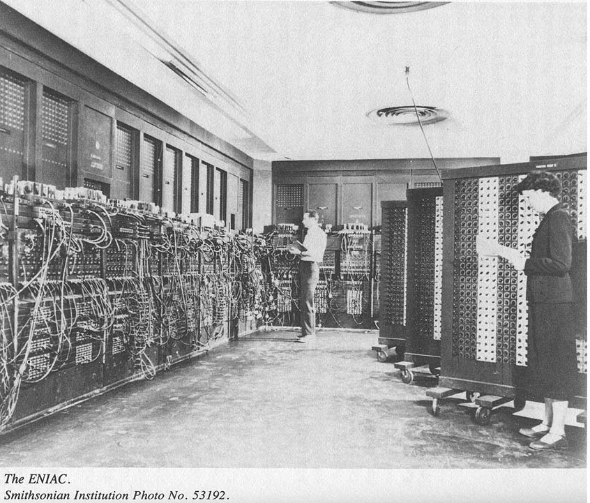
Physical
specifications:
40 panels, each 9' x 2' x 1', arranged in a U-shape; other units on casters could be positioned at various places. 18,000 tubes, 1,500 relays. 80 different DC voltages, ranging from -920 to + 550 volts; main power 240 volts, 60 Hz. Power consumption: 150 kW, 80 kW for tube heaters, 45 kW for other electronic circuits, 5 kW for input/output devices, 20 kW for ventilating and cooling.
Architecture: Word length: 10 decimal digits plus sign; ten's complement for negative numbers and subtraction; fixed decimal point-switch- selected; multiplication by table look-up. Addition and subtraction done in accumulators; separate unit for multiplication, division, and square-rooting. Other units for cycling (timing), pulse generation, and programming.
Reckoners, ENIAC, page 0124

Memory: 20 numbers in the accumulators: 100 read-only numbers in a function table; other storage by punched cards; also twenty 10-digit constant switches.
Speed: Pulse frequency, 100 kHz, or one pulse every 10 microseconds. Basic cycle was one addition time, 20 pulses, or 200 microseconds (5,000 additions/second).
Multiplication time, 14 addition times, or 2,800 microseconds (357 multiplications/second). Division time varied, up to 38 divisions/second. The ENIAC could be run at slower speeds, including a single pulse at a time, or a single cycle at a time, for diagnostic purposes.
Programming: Plugboards and switch settings. Full conditional branching and subroutine capability; also the ability to perform parallel sequences of operations. Slow to set up: a day or two for each new problem.
Input: 80-channel IBM punched-card reader; could read 2 numbers/second.
Output: Standard IBM printer. Each accumulator also had a bank of neon lights showing its contents; at normal speeds these were of course illegible, but at diagnostic speeds they could be read.
Miscellaneous: Much of the metalwork and other physical construction done by Livingston & Conway, Inc., a Philadelphia construction firm. Cooling system designed and built by Eggly Engineers, also of Philadelphia. RCA of Camden, New Jersey, supplied the tubes.

EVALUATION OF THE ENIAC

The ENIAC was a pioneering machine. But it had an inelegant design, was hard to program, had a limited memory capacity, and had slow input/output facilities. That much was frankly acknowledged by its builders in their reports on the machine written in 1945 as the machine was being completed.27

Those reports devote much space to the ENIAC's successor, the EDVAC, in which Eckert and Mauchly hoped to overcome most of the ENIAC's deficiencies. The EDVAC (Electronic Discrete VAriable Computer) would use binary arithmetic, would have a high-speed read-write memory of large capacity, and would execute programs that were internally stored in its memory.


Reckoners, ENIAC, page 0125

In the EDVAC there would also be a separation of memory functions and arithmetic. It needed a fast and large memory, which would be much more difficult to achieve if each memory cell also had to be capable of performing addition, as the ENIAC's accumulators did. Thus its designers returned to the overall structure for a computer that Charles Babbage had decided upon a hundred years earlier for his Analytical Engine (and which Konrad Zuse independently rediscovered in the late 1930's).

Aside from those design shortcomings, the ENIAC's biggest drawback was that it had far too many tubes. That was the chief reason why some government and military officials, including George Stibitz, were reluctant to fund the project at all. No one was sure that the ENIAC would run long enough between tube failures to do any useful work.28 Tubes are inherently less reliable than other electronic components; that is why they are not soldered into a circuit the way resistors or capacitors are, but are rather mounted in sockets for easy replacement. Even after the ENIAC was unveiled to the public and demonstrated its reliability, other computer designers (including Zuse and Aiken) continued to use the slower relay technology.

But the ENIAC was actually quite reliable in absolute terms, and much more reliable than the relay computers when its speed is taken into account. If the ENIAC could be made to run without a tube failure for only one hour, it could in that hour do more computing than the Bell Labs Model V could do in fifteen days of round-the-clock operation, based on their relative multiplication speeds. The claim that the relay computers could, and often were, operated unattended through the night (something the ENIAC never could do) must be tempered by that fact.

A graph of failure rates of electronic components looks like the letter U. Failure are high when the components are new, then follows a long period of trouble-free operation, followed by a gradual increase in failures as the components age. Whenever the ENIAC was turned on it would usually blow a tube. When a tube is cold, its filament has a different resistance and physical shape than when it is hot, so it is more likely to burn out when it is first turned on.29 So the ENIAC was hardly ever turned off. Surprisingly few cases of wiring mistakes turned up, and there were a few malfunctions due to "cold-soldered" connections, where the solder did not receive enough heat to form a good electrical bond. But those were quickly located and fixed.

After the tubes were left on all the time, the ENIAC could run about twenty hours between tube failures-a remarkably good record, due mainly to the conservative ratings at which the tubes and all other components in the computer were run. After it was moved from Philadelphia to Aberdeen, failures were more frequent, but eventually there, too, a good in-service record was established.

Besides the oft-mentioned fact that all the components were run well below their rated capacity, the design of the ENIAC was such that when a failure did occur, it could be isolated and repaired quickly. Indeed, at no time while it was in Philadelphia was the ENIAC ever shut down for more than a few days. The increased complexity of its design actually made it more reliable: by having a complicated power supply delivering many different voltages to the circuits, the machine could be run at slower speeds, down to one pulse at a time, to track down a problem. Neon bulbs revealed the contents of the accumulators; normally they blinked too fast to be readable but at single-step speeds they were.30


Reckoners, ENIAC, page 0126

The ENIAC's ring counters were designed to be unplugged as a unit. If one malfunctioned, an identical spare, known to be in good working order, could be plugged in, while the defective one was brought to a bench where it could be repaired without tying up the whole computer. This sort of "modular" approach to systems reliability is taken for granted in the computer industry today, but it was hardly known at that time.

There was no provision for the kind of elaborate internal checking pioneered by Bell Labs in their relay computers. Before working on a problem, at intervals during the solution, and after running the problem, its programmers ran special diagnostic programs to test the circuits.31

But it was still clear that the ENIAC had too many tubes. Eckert and Mauchly stressed that in the EDVAC they would have the same computing power with one-sixth the number of tubes. They had made the ENIAC a reliable computer, but just barely. In a sense the skeptics were right in being pessimistic about vacuum tubes. The reliability problem was always a serious one until tubes were replaced by transistors after 1960- thereby lifting the whole question of computer engineering, and with it reliability, to a new level of sophistication.

HOW THE MACHINE WAS USED

The acronym ENIAC stood for Electronic Numeric Integrator and Computer, and that is a good description of what kind of work it did. If Bessel functions were the Mark I's bread and butter, then the solution of differential equations by numeric methods was the ENIAC's. Its original goal was to compute and tabulate firing tables, and that goal remained central throughout its design, development, and construction. But the way it was built meant that it could do much more than that. By the time the computer was ready for testing late in 1945, the war was over, and the need for firing tables had lost some of its urgency; but that did not really matter. Differential equations of the kind encountered in ballistics are also found throughout physics, and if the ENIAC could be programmed to solve them, it would be kept busy.

The first problem it attacked linked the ENIAC with that other great project of the Second World War, the Manhattan Project. In July of 1945 the world's first atomic bomb exploded over the forbidding deserts of New Mexico. Building that bomb required, among many other things, a lot of computation. Its fissionable material was ignited by an implosion of a carefully shaped and timed firing of TNT, and the scientists who designed it had to calculate the geometry of the shock wave to an exacting tolerance. Most of the computing at Los Alamos was done by mechanical desk calculators and IBM punched card equipment.


Reckoners, ENIAC, page 0127

But even as the atomic explosions at Hiroshima and Nagasaki hastened the end of the war, the scientists at Los Alamos were looking toward the hydrogen bomb, the "Super," which would have a much higher yield than the fission bomb. Designing it required even more calculations, far too many to be done manually or even with an electromechanical computer. Right then along came news of the ENIAC's nearing completion. Nicholas Metropolis and Stanley Frankel went to Philadelphia late in 1945 and arranged that the first problem the ENIAC would run would be a classified problem to test the feasibility of the Super's design.32 Few people at the Moore School, including Eckert and Mauchly, could even be told of the nature of the problem, but of course they were given the mathematical equations the ENIAC was to solve. It was a very large partial differential equation whose set-up required a million punched cards for input and transfer of numeric data. The problem overwhelmed the ENIAC's internal memory, so it was divided into sections, with intermediate results punched onto cards and reentered into the machine.

The ENIAC solved the problem-without ever having the chance to go through any shakedown or test phase. Actually, the Super computation was the shakedown cruise for the ENIAC. Right from the beginning it proved itself to be a fine machine indeed.33 The problem itself remains classified to this day, but it is known that the answer computed by the ENIAC showed that the Super would not work as designed. It was a design based on freezing the heavier isotopes of hydrogen and detonating them by the compression from a fission bomb. Even after the negative results of the ENIAC's computation, a test of the so-called wet bomb design was conducted at Eniwetok in the Pacific in 1951. In that test, fusions of hydrogen nuclei did take place, but there was no thermonuclear explosion. (Early in 1951, Stanislaw Ulam and Edward Teller conceived of a different approach, one using not the blast wave but rather the x-ray emission of the fission bomb to fuse the hydrogen. That approach led to America's first hydrogen bomb shortly thereafter.)

The ENIAC proved its worth so quickly that it was busy from that moment on. There never was any time for testing or "running in" the machine. Its move to Aberdeen was postponed until late 1946 because of the urgency of the first problems it solved. When it finally was moved, it was turned off in November, 1946, and not started up again until late summer, 1947. So for most of the year 1947 the world had to get along once again without any electronic numeric computers.

Questions of whether or not the ENIAC was truly a general-purpose numeric computer are best answered by looking at some of the problems it did in that first year. Herman Goldstine, who with his wife Adele did much of the programming of the ENIAC, has documented problems in computing tables of trigonometric series, another simulation of a nuclear reaction, problems concerning the propagation of shock waves in compressible fluids, and even a problem in number theory submitted by D. H. Lehmer. The ENIAC also tackled a problem in weather forecasting-Mauchly's old dream-though it was not Mauchly but John von Neumann who submitted it.


Reckoners, ENIAC, page 0128

The British physicist D. R. Hartree used the ENIAC between April and July, 1946, for a problem involving the flow of a compressible fluid over a surface, such as air over the surface of a wing travelling faster than the speed of sound. Hartree had already used the Differential Analyzer for that problem. He found the ENIAC's memory too limited for its solution by an iterative method, but he tried a different approach more suitable for the ENIAC's structure, and it worked well. He divided the area to be computed into 250 intervals, and the machine computed and punched answers to seven-place decimal accuracy.

Hartree's work is especially interesting because it was a full-scale problem that taxed the ENIAC's full capabilities, but it was not a ballistics calculation. Although it involved the numerical solution of an ordinary differential equation, its set-up was very different from the kinds of set-ups Eckert and Mauchly had envisioned for computing firing tables. So from the very beginning, the ENIAC showed that it had a broad range of applicability.34 Another consequence of Hartree's work was that he published an account of it in a series of notes in the British journal Nature, in 1946, as well as in a longer paper in the Philosophical Transactions of the Royal Society in 1948. Those articles helped publicize the speed and power of the new invention. In general, the ENIAC never strayed far from numerical integration of differential equations. That was what it did best. But at least it could do other things, easily enough for some persons to make the attempt. After it was installed at Aberdeen, it finally got a chance to compute firing tables, which it did reliably and well for many years.

By the end of 1945 the new computer had scarcely begun running, yet it was already clear that the whole project was going to be a success. The war was over, and those who had been working so hard on the computer wanted to share their excitement with others. A public dedication was held in February, 1946, during which the machine demonstrated its ability to sum and multiply numbers at speeds few people could adequately comprehend. Representatives of the press watched as the machine computed a full trajectory in twenty seconds-faster than the shell itself travelled from the gun to its target. That seems like a silly comparison by today's standards of measuring computer speeds, but it was enough to convince the more skeptical members of the audience.

With the lifting of wartime secrecy the development of the digital computer entered a new phase. Communication barriers were not lifted entirely or immediately, but the published descriptions of the various projects meant that subsequent computer projects would proceed more along common lines. The "pre-historic" age ended, and there followed a more direct line of descent to the present day. From 1945 to 1950 a consensus emerged: the computer's future lay in machines that were electronic, not electromechanical, and digital, not analog. They would compute in the binary scale, and they would have as much high-speed read-write memory as possible. The memory would be restricted to storage and retrieval of data; all arithmetic would be concentrated in a separate unit specially built for that purpose. Most important, future computers would store not only numerical data but also their own programs in that same internal high-speed memory. How those concepts, especially the last one, emerged, will be discussed next.


NOTES

  1. 1. J. Good, "Early Work on Computers at Bletchly," Cryptologiia, 3 (1979), 65-77; Simon Lavington, Early British Computers (Bedford, Mass.: Digital Press, 1980), Chapters 1, 2.
    Reckoners, ENIAC, page 0129

  2. Cuthbert Hurd, "Early IBM Computers: Edited Testimony," Annals of the History of Computing, 3 (1981), 163-182.
  3. Herman H. Goldstine, The Computer from Pascal to von Neumann (Princeton: Princeton University Press, 1972), Part Two; Nancy Stern, From ENIAC to UNIVAC (Bedford, Mass: Digital Press, 1981); Arthur Burks, "The ENIAC: First General-Purpose Electronic Computer," Annals of the History of Computing, 3 (1981), 310-389.
  4. John Brainerd, "Genesis of the ENIAC," Technology and Culture, 17 (1976), 482-488; Goldstine, Computer, pp. 127-139.
  5. Gilbert A. Bliss, Mathematics for Exterior Ballistics (New York, 1944); Edward McShane, John Kelley, and Franklin Reno, Exterior Ballistics (Denver: University of Denver Press, 1953), especially the Appendix on its history, pp. 742-799; Forest Moulton, New Methods in Exterior Ballistics (Chicago: University of Chicago Press, 1926); Thomas J. Hayes, Exterior Ballistics (New York: Wiley, 1938).
  6. Goldstine, Computer, pp. 146, 137-138.
  7. Burks, "The ENIAC."
  8. John Mauchly, "The ENIAC," in N. Metropolis, J. Howlett, and G. -C. Rota, eds., A History of Computing in the Twentieth Century (New York: Academic Press, 1980), pp. 541- 550.
  9. Nancy Stern, "From ENIAC to UNIVAC: A Case Study in the History of Technology," Dissertation, SUNY, Stony Brook, New York, 1978, pp. 41-48; Goldstine, Computer, p. 150.
  10. Nancy Stern, "John W. Mauchly: 1907-1980," Annals of the History of Computing, 2 (1980), 100-103; Lewis F. Richardson, Weather Prediction by Numerical Methods (Cambridge, England, 1922).
  11. Burks, "The ENIAC"; letter from John V. Atanasoff to the author, May 25, 1980; for an example of a special-purpose mechanical device that solved systems of linear equations, see the description of the "Wilbur Equation-solver" in Charles and Ray Eames, A Computer Perspective (Cambridge, Mass.: Harvard), p. 113.
  12. The Industrial Reorganization Act: Hearings Before the Subcommittee of the Judiciary, U.S. Senate, 93rd Congress, Part 7: The Computer Industry, July 23-26, 1974; Earl R. Larson, Findings of Fact, Conclusions of Law and Order for Judgement, File No. 4-67 Civ. 138, Honeywell, Inc., vs. Sperry Rand Corporation and Illinois Scientific Developments, Inc., U.S. District Court, District of Minnesota, Fourth Division, October 19, 1973.
  13. H. J. Reich, "Trigger Circuits," Electronics, August, 1939, pp. 14-17; Hurd, "IBM Computers"; W. H. Eccles and F. W. Jordan, "A Trigger Relay Utilising ThreeElement Thermionic Vacuum Tubes," The Radio Review, 1 (1919), 143-146.
  14. J. Presper Eckert, "The ENIAC," in Metropolis, Howlett, and Rota, A History of Computing, pp. 525-539; Mauchly, "The ENIAC," in Metropolis, Howlett, and Rota, pp. 541- 550; J. Presper Eckert, "A Survey of Digital Computer Memory Systems," Proceedings, IRE, 41 (1953), 1393-1406.
  15. Arthur Burks, "Computing Circuits of the ENIAC," Proceedings, IRE, 35 (1947), 756- 767.
  16. Eckert, "Survey of Memory Systems."
  17. Eckert, "Survey of Memory Systems"; Mauchly, "The ENIAC."
  18. Burks, "Computing Circuits of the ENIAC"; Burks, "The ENIAC."
  19. For a popular account of the Colossus, based on interviews with some of the participants, see Christopher Evans, The Micro Millennium (New York, 1980), pp. 34-36. Evans's interviews are available as the "Pioneers of Computing" series from the Science Museum, London.
    Reckoners, ENIAC, page 0130

  20. Burks, "Computing Circuits"; J. G. Brainerd and T. K. Sharpless, "The ENIAC," Electrical Engineering (February, 1948), pp. 163-172; J. P. Eckert, et al., "Electronic Numerical Integrator and Computer," U.S. Patent No. 3,120,606 (June 26, 1947); Herman Goldstine and Adele Goldstine, "The Electronic Numerical Integrator and Computer," Mathematical Tables and Other Aids to Computation, 2 (1946), 97-110.
  21. D. H. Lehmer, "A History of the Sieve Process," in A History of Computing in the Twentieth Century, N. Metropolis, J. Howlett, and G. -C. Rota, eds. (New York: Academic Press, 1980), pp. 445-456.
  22. U.S. National Defense Research Committee, Applied Mathematics Panel, "De scription of the ENIAC and Comments on Electronic Computing Machines," Report 171.28, November 30, 1945.
  23. Franz Alt, "A Bell Laboratories Computing Machine, Part II," in Brian Randell, ed., Origins of Digital Computers, p. 527.
  24. John Mauchly, "Preparation of Problems for EDVAC-type Machines," in Randell, Origins, p. 366.
  25. Burks, "Computing Circuits of the ENIAC"; National Defense Research Commit tee, "Description of the ENIAC," p. 3/9; N. Metropolis and W. J. Worlton, "A Trilogy on Errors in the History of Computing," First USA-Japan Computer Conference, October 3-5, 1972 (Tokyo), pp. 683-691; J. P. Eckert, "ENIAC," in Metropolis, Howlett, and Rota, History of Computing.
  26. For this and the following descriptions of the ENIAC's structure I have relied mostly on Burks, "The ENIAC," cited above.
  27. National Defense Research Committee, "Description of the ENIAC," pp. 2/4-2/5, also section 4.
  28. J. Presper Eckert, "Thoughts on the History of Computing," Computer (Decem ber, 1976), pp. 58-65.
  29. Goldstine, The Computer, p. 145; Brainerd and Sharpless, "The ENIAC," pp. 168-169.
  30. Industrial Reorganization Act, p. 5810; Eckert, "Survey of Digital Memory," p. 1394.
  31. Brainerd and Sharpless, "The ENIAC," p. 169.
  32. Burks, "The ENIAC."
  33. Nancy Stern, ENIAC to UNIVAC, pp. 62-63; Goldstine, The Computer, p. 234.
  34. Hartree published several accounts of his experience with the ENIAC: "The ENIAC: An Electronic Computing Machine," Nature, 157 (April 20, 1946), p. 527; and 158 (October 12, 1946), pp. 500-506; a description of the problem he ran on it appears in Calculating Instruments and Machines (Urbana: University of Illinois Press, 1949).


Go Forward, Go Back, Go to Table of Contents, Go to On Line Documents, Go to Go to Antique Computer home page