An idea of the power (speed) of Babbage's Difference Engine
from Tim Coslett
It seems that the Babbage machine (mechanical, designed about 1848) is about as fast as the ENIAC (electronic, designed and built about 100 years later) on this particular problem. |
The Goal of this document is to provide you with the knowledge and
computational tools (including free downloadable
extended precision UBASIC and an On-Line Manual)
(easier to use)
so that you can initialize and
emulate the Babbage Difference Engine #2 to:
* Please note, this JavaScript emulator fails to run properly on Internet Explorer 7 and up. Disclaimer - I (the author of this piece) am neither a mathematician nor historian (I are a enjineer!)
The Goal of the Babbage Difference Engine was to provide accurate trig and log tables (for navigation, engineering & astronomical computations). Babbage designed this version of difference engine during 1847-1849, using technical improvements discovered while he was designing his Analytical Engine. One can think of Babbage's Difference Engine as a means of providing an interpolation between widely spaced known points. To use the available power (seventh degree polynomial) of the engine, eight known points are required. Two of the points near the end points of the function to be approximated, and six points roughly evenly spaced in-between the end points.
This web site also includes two manuals kindly provided by British National Museum of Science and Industry
An article "Babbage's Expectations for his Engines" is also provided. |
|
Please note: This paper does not discuss the Babbage Analytical Engine
that contains many of the ideas of the modern computer, and was
described by "Ada King, Countess of Lovelace"
(please see name discussion here)
and others. The Analytical Engine development came
after the construction of the Difference Engine was abandoned.
The design of Difference Engine II incorporated improvements found during Babbage's design work on his Analytical Engine - yielding a reduction of parts count from 25,000 to 8,000. For the Babbage Analytical Engine, here is Charles Babbage -- Scientist and Philosopher and an interesting web site. |
This paper is organized into the following sections
- A short introduction
- Eight pages of an 1822 Babbage letter describing the error problem and his solution
- How the French (and most others?) calculated math tables in the early 1800s
- Examples of formulas for trig and log values
- Method of Finite Differences saves labor when making tables
- A simple example of the
Method of Finite Differences
- also see "Specimen Tables, The Swedish Calculating Machine" by Scheutz (Google books) - Why Simple Differences does not work well with Trig & Log tables
- The Interpolating Polynomial
A polynomial of limited degree that approximates the desired function - Forming the Interpolating Polynomial
- Finding the Differences using the Interpolating Polynomial
- Scaling to permit dealing with fractions (or approximations to fractions like 1/3)
- Representing negative numbers, (10's complement)
- Correcting the initialization for the Babbage odd-even parallel pipelined operation
- Setting up the engine, Babbage Difference Engine #2 Instruction Manual
- Some computed example results
- A good machine test case
- a JavaScript non-pipelined emulation
another simulation starting (alpha version) by Nathan Lisgo @nlisgo (https://twitter.com/#!/nlisgo) and Paul Martin. - A (mercifully) short discussion on computing errors
- Babbage Overflow-Underflow detection
- Formatting the output of the Babbage printer section.
- Some Babbage websites
- Some Babbage on line books other sites
- Some Babbage books
- Serious comments about Babbage's design.
- SetUp Script for setting coefficients in the for Babbage Engine #2, Second Edition ;-))
Assume a polynomial of degree 7 (above) or less, with integer coefficients
(a, b, c, ... are integers).
If you set up a Difference Engine correctly, (insert the correct things to add)
the Difference Engine will evaluate the polynomial (give y) for successive integer values
of x until the machine overflows (numbers get larger than the machine
can handle).
This is interesting, but even more interesting is the
fact that if you form a polynomial that approximates (or interpolates) a function
(say the sine function), the Difference Engine will evaluate the
(sine) function to arbitrary accuracy (such as 15 digits).
This is useful in making those boring trig tables so necessary before electronic calculators which calculates functions only as needed.
The British needed accurate trig and other tables for navigation of their sea going
merchant and naval vessels. They
were very interested in such developments and machines in the 1600s through the 1800s.
Babbage had investigated errors in navigational and astronomical tables,
and realized that both correct
computation and printing were needed. So the second part of
his Difference Engine was a type-setting machine, which reduced the probability
of human error to a minimum.
He was awarded a gold metal by the British Astronomical Society for his paper
"Observations on the Application of Machinery to the Computation of Mathematical Tables."
in 1821.
Charles Babbage was an interesting character; very gifted, but he was
a very poor project engineer and politician.
This paper is not about him or his problems and failure in producing
his Difference Engine, but is about how to set up a Difference Engine # 2 so that it
can produce the desired tables.
Examples of series expansion
cos x = 1 - x2/(2!) - x4/(4!) - x6/(6!) + ...
ex = 1 + x + - x2/(2!) - x3/(3!) - x4/(4!)
+ ...
Logex = (x - 1) - (1/2)*(x - 1)2 +
(1/3)*(x - 1)3 - ...
For more examples, and a good discussion see
this Wikipedia section.
Half angle formulas, starting at known points such as sin 30 degrees = 0.5, sin 45 degrees = 0.5*SQRT(3)
More on
half angle formulas.
The above formulas CAN be used to compute each entry in the tables of sin, cos, ...
But for tables, not much used these happy electronic days, other methods were used
to save arithmetic operation,
The "Method of Differences", dear to the hearts of Numerical Analyst's, saves
an enormous amount of arithmetic, especially multiplications and divisions whch
are much more labor intensive than additions.
You will note below that to compute the next value (x = x + 1) for a polynomial, the only
processing required is a number of additions equal to the degree of the
polynomial. An example, a 7th order polynomial (shown above)
requires just 7 additions for each successive value of x.
Using above difference values to calculate y = x3
The difference values obtained by the above process (0, 1, 6, 6, and 0)
note: the noun "Difference Column" has been abreviated to "DC" in the table below.
adding DC1 to DC0, then DC2 to DC1, ...
Summary of the above difference method. A polynomial of limited degree
(number of terms, power of exponents, ...) can be evaluated exactly to many values
of x by using the method of differences. In the method of differences, you
evaluate a few values of x, do the differences, and by simple addition, and
can evaluate a large number of values.
Unfortunately, trig and log functions are not low order polynomials with integer coefficients.
In fact, trig and log functions are NOT polynomials, but irrational, transcendental functions.
The method of differences works exactly for the number of terms used to
compute the differences, but begins to fail on succeeding cycles. The Taylor
series for sin:
has just 4 derivatives in the range to the seventh power.
Using the method of finite differences for the first 8 increments provides
perfect results (duplicates the inputs) for the 8 iterations, but begins to
deviate significantly after a number of iterations.
The differences depend upon the relative range of the difference sample
versus the range of the desired calculations. In a
MATHEMATICA example
and a
UBASIC example
using the sin function,
0 to 7 degrees were used, and the desired range was 45 degrees. The error at
the far end of the range (45 degrees) approaches 0.0001 percent.
This is just a table of 45 values - trivial - and the errors are almost intolerable already.
HOWEVER - in a more useful sin table, with a value every 1 minute, things go
dramatically wrong using this simple method. See this
UBASIC example of a sin table with an output every 1 minute
of angle.
To summarize, if you are forming trig and log tables, using the method that works
so well with polynomials of 7th degree or less fails. The first 8 values have 0 error,
then the rest of the values have increasingly bad errors.
In the next section, we will examine a method where few if any values are EXACTLY
correct, but all values are within known (and hopefully acceptable) error limits.
Fortunately there is a good "work around" to the fact that some of the most desirable
functions are not polynomials. You can form a polynomial
that approximates the function (example sine) to high precision (say 15 digits) over the
range of interest (say 0 to 45 degrees) and accept that most values in that range
will not be "perfect". But the values can be within the allowed error tolerance,
say 15 decimal digits. If you print the table accurate to 15 decimal digits, everyone will
be satisfied - actually happy.
This page (750 KB) from "Applied Numerical Methods"
by Carnahan shows that "least squares curve fit" is not needed when exact points are available.
The higher the order of the polynomial, the closer you can "fit" the
polynomial to the desired function. Unfortunately, the higher the
order of the polynomial, the more expensive the computing machine.
In these days of wonderfully cheap computing capability, you could
choose a 100th degrees polynomial with no visible impact on your budget.
However, Babbage was making his machine from very expensive precision
machinery, and he had to compromise. His compromise, which was still
too expensive to attract investment money - was a 7th degree polynomial design.
The same cost driven compromise caused Babbage to restrict the precision
of the Difference Engine to 31 decimal places. This seems like an
excessive precision - BUT - a wide variety of error sources, which
accumulate in the calculations, are caused by a finite limit to the computing accuracy.
AND several digit positions of the machine are need to count operations to provide
the "argument" column of the printed table, such as from above
y = x3 example.
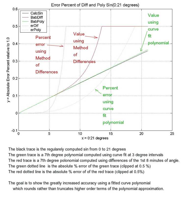
Fortunately, you can reduce the errors caused by the missing higher order terms by
adjusting the available (7th order) terms by closely fitting a lower order (7th order)
polynomial as closely as practical to the function over the range of interest.
(And if the errors are too great, you can reduce the range and reduce the errors.)
Curve fitting the approximating polynomial to the actual function helps correct for
the missing higher order terms of the actual function.
The individual values of the approximating polynomial, while not usually perfect,
can closely approximate the function over the entire desired range. I will show that
by using just a 7th order "interpolating polynomial" the sin function can be computed
in 1 minute steps from 0 to 23 degrees (1860 steps) with a maximum error of
10-12. With this kind of accuracy, if every thing else is perfect,
a navigator can determine his position within an inch relative to the earth's surface.
That ought to be good enough, even for the British Navy. ;-))
Now, how to make a polynomial from the sine trig function.
For instance, the sine (and cosine) of 45 degrees is 1/(square root of 2) exactly so
using half angle formulas the angles
And using the sum of angles formula
To save error prone manual copying, there is a "copy" available in the
"Edit" button that copies to the "clipboard" and you can copy the
clipboard value to an editor or some curve-fit programs.
Here is an
example,
written in MATHEMATICA (a wonderful and expensive extended precision
mathematical tool - I have a very old student version). The extended precision is needed
as IEEE floating point used by many low cost or free tools, such as Euler
is accurate to "only" 15 decimal digits. Since the Babbage machine is capable of
up to 31 digit precision, errors due to the limited precision of the floating point
other packages introduces serious simulation errors.
Unfortunately, the above packages are not free - even student versions
are sold for about $140.
A handy 15 decimal digit accuracy curve fit package is found at
the web site
of John Kennedy, retired
mathematics instructor from Santa Monica College.
Make a new directory, then access
John Kennedy's web site,
click on "Downloadable Math Software", then download "JK32W2.ZIP" to your new directory.
(I am assuming that you have access to PKZIP or a similar expansion routine.)
Unzip the file, and Start polyfit.exe. This starts a handy Windows program
that can calculate "Least Squares Fit" of data to the limits of IEEE floating point.
Using the above coefficients, do the following
Yielding the
table 0-2 degrees 8 K bytes,
table 0-23 degrees 88 K bytes,
and a
table with errors
Scaling is multiplying or dividing a variable by some constant so that you can make it fit
into your computing machine. It is a little like the U.S. government budget.
We humans divide all the numbers by say a million or a billion so we can think
of them in our rather limited minds. Computers are also limited
in the size and precision of the numbers they can handle naturally.
(Humans can write and add numbers as large as they wish, limited only by the
size of the sheet of paper and the time you wish to spend.
You can write down 2 one-hundred digit numbers just fine, and add them with no problem.
However, a one-hundred digit number in meaningless to most of us - just HUGE!)
Most modern machines, for reasons of economy and speed, work naturally with a few sizes of
numbers. A 2 byte word can represent numbers within the range of about +- 32,000,
about 4 decimal digits of precision.
A 4 byte word can represent numbers with a range of about +- 2,000,000,000,
about 9 decimal digits
of precision.
The most usual "scientific" floating point has about 15 decimal digits of precision,
and an automatic method of sliding the decimal point around in a handy fashion.
All of the above have a handy way of detecting "overflow" or "underflow" where the
correct answer after an arithmetic operation cannot fit into the defined number range.
The Babbage Difference Engine #2 represents numbers as 31 decimal digits,
greater precision than "natural" in modern machines. But even 31 decimal digits precision
cannot exactly represent the fraction one/three or 1/3 that we can approximate as
0.333333333333333333... .
Let us assume the decimal point to the right of a computer number, and add
HOWEVER, if we multiplied the factors by say 1,000,000,000 we get
This multiplying of variables by a constant to fit the machine is one usage of scaling and is used a great deal in Babbage and in modern machines.
A major advantage of using floating point
arithmetic and hardware, included in most machines in our current era
of almost free logic, is to reduce the need for, and human errors in estimating, scaling.
To do the equivalent with a machine takes extra hardware and (possibly more important)
time. By custom hardware representation of negative numbers is made such that
you can add or subtract numbers (quickly & cheaply) and not even know or care about the sign.
In most machines, a negative number is represented as though you took the absolute value
of the negative number and subtracted it from the largest value the
machine can represent, and then adding the smallest positive number the machine can
represent. This is called 10s (or 2s) complement.
An example is a little easier to see, we have say -3. The absolute value is
Adding +5 to the -3 above yields
10s (or 2s) complement arithmetic is a little tough for humans, but fast and simple
for machines - so 10s (or 2s) complement inside, converted to the other form out side
the machine for us slow humans.
Unfortunately, to set up a Babbage machine, you must set the rotors
for 10s complement arithmetic - the negative numbers "look funny".
HOWEVER, the print subroutines I provide in TOOLS output 10s complement values.
The goal of this section is to make the output of the Babbage machine identical
with the ouputs of section 6. "A simple example of the Method of Finite Differences"
above.
----- Correcting for printing after the adds
Fortunately, there is a simple solution for the above situation. This BASIC code
shows how to back up the input one step so that the expected results will be output.
----- Correcting for the odd-even phasing of adds
The names of the difference columns are taken from the conventions in section 6 above.
The "Technical Description Manual",
page 66 uses different Difference Column numbers, which we will ignore to reduce confusion.
The initialization must be adjusted to allow for this even-odd, parallel,
"pipeline" operation. In the notation below,
Unfortunately, the simple difference set up used in the Normal serial operation
does not work for the Babbage parallel operation - expected operations are
done out of sequence, and the results are just wrong.
To correct the parameters set into the Babbage machine, you MUST
Subtract various differences. Perform the following in exactly this order.
A code example and output is here.
1. A short introduction
The Babbage Difference Engine is basically a fancy adding machine that can do
unexpected (amazing) things with polynomials. An example of a polynomial is
Shown here are two pages (of 390 pages) from a modern book of mathematical tables
- "Mathematical Tables"
published by "Chemical Rubber Publishing Co." in 1948
This book also contains logs of trig functions, Gamma functions,
hyperbolic functions, and much much more.
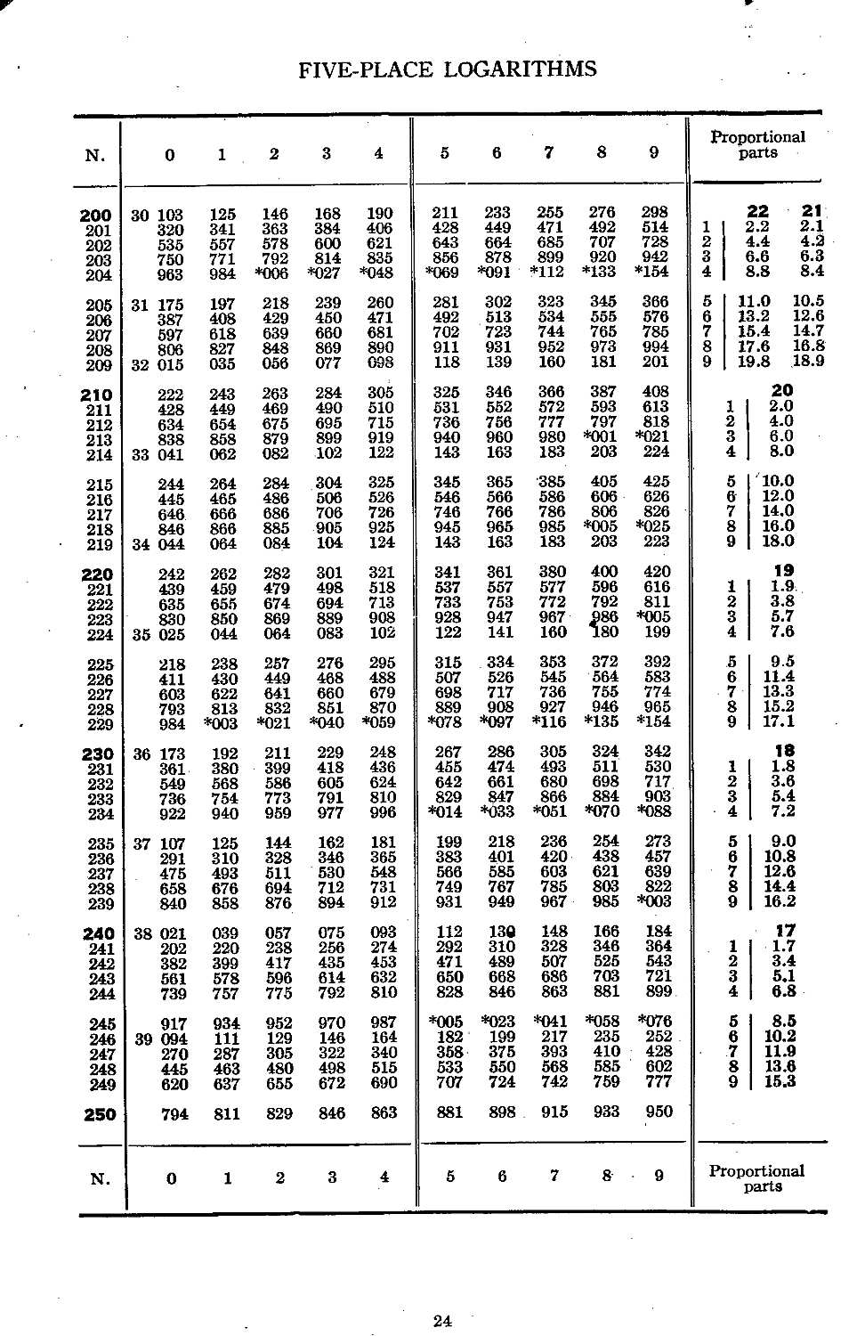
This is one page (of 18 pages) of the five-place logarithms - from 200 through 250

This is a page of natural trigonometeric functions - from 28 through 29 degrees.
2. Eight pages of an
1822 Babbage letter describing the error problem
and his solution
3. How the French (and most others?) calculated
math tables in the early 1800s
4. Examples of formulas for trig and log values
sin x = x - x3/(3!) + x5/(5!) - x7/(7!) + ...
where (2 > x > 0)
Nicolaus Copernicus used half angle formulas to compute his tables to 10 minutes of angle.
The user interpolated for intermediate angles.
sin 0.5x = +-SQRT((1-cos x)/2)
cos 0.5x = +- SQRT((1+cos x)/2)
- Table in "On the Shoulders of Giants" by Steven Hawking, page 44 ...
5. Method of Finite Differences saves labor when making tables
HOWEVER,
the cost in terms of computation was excessive in the days of hand calculations.
Your modern hand calculator (and personal computer) calculate the instances
of these functions using formulas similar to the above formulas carefully modified
to require a minimum of terms to attain the required results.
6. A simple example of the Method of Finite Differences
- also see "Specimen Tables, The Swedish Calculating Machine" by Scheutz (Google books)
Bolded numbers below are difference values obtained by the process
Method of Finite Differences for y = x3
The symbol -> indicates subtract the number just above from the number just below and place the result to the right.
x (cycle) y = x3 1st dif 2nd dif 3rd dif 4th dif
0 0
-> 1
1 1 -> 6
-> 7 -> 6
2 8 -> 12 -> 0
-> 19 -> 6
3 27 -> 18 -> 0
-> 37 -> 6
4 64 -> 24
-> 61
5 125
are placed into the Difference Columns of a "difference engine".
cycle
(x)DC0
(y=x3) DC1 DC2 DC3 DC4
0
0 1 6 6 0
1
1 7 12 6 0
2
8 19 18 6 0
3
27 37 24 6 0
4
64 61 30 6 0
5
125 91 36 6 0
6
216 127 42 6 0
7
343 169 48 6 0
An example of the above, and the BASIC program, is provided
here
7. Why Simple Differences does not work well with Trig & Log tables -
The above simple system works perfectly with a polynomial of a limited number of terms
with integer coefficients.
By the way, you notice that I make a big deal about extended precision. there is an
example of using normal IEEE floating point (about 15 digit precision). You may notice that
similar code to the example in the above paragraph yields an error of 54% at a mere 12 degrees.
8. The Interpolating Polynomial
A polynomial of limited degree that approximates the desired function
x y = x3
0 0
1 1
2 8
3 27
4 64
5 125
6 216
7 343
9. Forming the Interpolating Polynomial
We now have the coefficients, accurate to about 31 decimal places, of the sine function
over the range of 0 to 23 degrees.
Of course, Nicolaus Copernicus and Isaac Newton did not have handy calculators. However they could get a
nice selection of numbers using symmetry formulas
here
The "half angle" and "sum of angles" formulas are of particular interest.
45, 22.5, 11.25, 5.625, 2.8125, ...
are available using the half angle formula
( sin(a/2) = SquareRoot((1-cos(a))/2) )
( sin(a+b) = sin(a)cos(b) + cos(a)sin(b) )
yields values for
2.8125, 5.625, 8.4375, 11.25, 14.0625, 16.875, 19.6875, 22.5 degrees.
And of course, the sine of 0 degrees is 0.0
	degrees  value of sin
	-------  ------------
	    0,   0
	    3,   0.052335956 2429438327 2211862960 90784
	    6,   0.104528463 2676534713 9983415480 2498
	    9,   0.156434465 0402308690 1010531946 7167
	   12,   0.207911690 8177593371 0174228440 5125
	   15,   0.258819045 1025207623 4889883762 4048
	   18,   0.309016994 3749474241 0229341718 2819
	   21,   0.358367949 5453002734 8413778941 3467
	   24,   0.406736643 0758002077 5398599034 1498
	     -  1.011225786 6802907976 5083139397  *1012
	     +  0.017453292 5216557274 7695492508  *x1
	     -  9.650085084 7235102648 2968837056  *1013*x2
	     -  8.860959019 0158230245 8402902990  *107*x3
	     -  3.559895737 1823585126 5053546540  *1014*x4
	     +  1.349880364 7432610642 7099346582  *1011*x5
	     -  1.182215638 0312276038 2796654565  *1016*x6
	     -  9.563667920 8157451630 8224691444  *1017*x7
	Coefficient	        Term
	--------------------    -----
	-9.28351019821882E-16	constant
	 0.0174532925208996	x
	-7.57903133381811E-13	x2
	-8.86095929472524E-07	x3
	-3.36840732998678E-14	x4
	 1.34987376001792E-11	x5
	-1.17367893545279E-16	x6
	-9.56350174721563E-17	x7
For your convenience, I have included John Kennedy's POLYFIT directory here.
You should be able to click on the .pdf and .txt files to see the contents.
To run PolyFit.exe , copy it to a directory, and click on it there -
10. Finding the Differences using the Interpolating Polynomial
11. Scaling to permit dealing with fractions
plus
generating
No problem, however if we do the division, and keep the decimal point on the right,
divided by
generating
clearly incorrect - the fractional part disappeared off to the right and is lost.
divided by
generating
Clearly a better approximation :-)
12. Representing negative numbers, (10's complement)
Human notation for negative number is usually a minus sign followed
by the absolute value the number. This is very convenient for humans,
"no problem". :-) A human eye can scan the number field and easily
detect the sign of the number, and based on the sign of the number, "do the right thing".
subtract the above from
generating
adding
generates
with the high digit not zero indicating that the number is negative
plus
generates
and the high digit is zero indicating positive.
13. The parallel "pipeline" nature of the Babbage machine and:
----- Correcting for printing after the adds
----- Correcting for the odd-even phasing of adds
Dick Guertin noted that data for the printer is taken from
DC0 during the 2nd half cycle, after an add into DC0, not the 1st half cycle. Thanks Dick
for I = 6 to 0 step -1
    DC(i) = DC(i) - DC(i+1)
next i
To save cranking, and to speed operations, the Babbage machine is arranged for
parallel "pipeline" operation.
DC0+=DC1 means add DC1 to DC0
Normal serial operation (Babbage outputs to printer at the end)

         DC0+=DC1
              DC1+=DC2
                   DC2+=DC3
                        DC3+=DC4
                             DC4+=DC5
                                  DC5+=DC6
                                       DC6+=DC7
Printer<- DC0        (copy DC0 to the printer)


The above could easily take 8 machine cycles

HOWEVER, as discussed in the "Technical Description Manual"
Babbage does as much as possible in parallel - called "pipelining"

Babbage pipeline - First half cycle
         DC0+=DC1  DC2+=DC3  DC4+=DC5  DC6+=DC7
Babbage pipeline - Second half cycle

              DC1+=DC2  DC3+=DC4  DC5+=DC6
Printer<- DC0        (copy DC0 to the printer)
for I = 6 to 0 step -1
    DC(i) = DC(i) - DC(i+1)
next i
     DC6=DC6-DC7  ' back off iteration 3, 1st half cycle
     DC5=DC5-DC6  ' back off iteration 2, 2nd half cycle
     DC6=DC6-DC7  '                     , 1st half cycle
     DC4=DC4-DC5
     DC3=DC3-DC4  ' back off iteration 1, 2nd half cycle
     DC5=DC5-DC6
     DC2=DC2-DC3  '                     , 1st half cycle
     DC4=DC4-DC5
     DC6=DC6-DC7
Using the above recipe, inserting these values into the machine (see section below),
and adding paper and ink, the Babbage Difference Engine #2 is ready to
compute and print your polynomial.
14. Setting up the engine,
Babbage Difference Engine #2 Instruction Manual
15. Some computed example results
16. A good machine test case y = K * x7
through the range -70 < x < 70
UBASIC code and results
MATHEMATICA code and results