From FM 44-1-2 ADA Reference Handbook, 15 June 1984, see page 21 "Rings of Supersonic Steel"
Return to home page, Goto Next Section
|
Wikipedia has a good article on the
History of Radar
so that defensive forces can detect and track aircraft - at greater distances - at night and through smoke, haze and clouds - obtaining accurate range |
This information is grouped into the following sections:
"RADAR" is a short form of the name "RAdio Detection And Ranging".
Basically:
- A radar set transmits radio waves out in a narrow beam (similar to a flash light beam).
- Some of the wave may hit an object and be reflected back (as an echo).
- Some of the echo is caught, amplified, and displayed by the radar set receiver.
- The time delay of the echo indicates the distance to the object.
The direction of the beam indicates the direction of the object.- The receiver displays the return signal on a display, with the echo as a bright spot or a raised blip.
Some available documentation
- An on-line Army manual "Introduction to Radar" ST-44-188-1 is available.
- An on-line Navy manual 2013 Electronic Warfare and Radar Systems - Engineering Handbook spotted by Greg Brown.
The jamming sections of this handbook.- A 2009 civilian presentation 1) ìRadar Basicsî, 2) "Radar Setsì, 3) ìAntennae Techniquesî, 4) ìRadar Transmitterî, 5) ìVelocity-modulated Tubesî,
There are two major types of radars, "pulse radar" and "continuous wave (Doppler) radar". (There is also a hybrid between the two sometimes called "Pulse-Doppler" used in Patriot radar. [thanks to Doyle Piland ])
(Also from Doyle Piland )
Chirp is another technology which is also used with pulsed radar. The general idea is to take advantage of the high power contained in a long pulse and still retain the range resolution of a short pulse. There are also other side advantages which makes it harder to use ECM against. Chirp simply uses a swept frequency, long pulse of up to 120 microseconds. I think the convention is the beginning of the pulse is the lower frequency and the high frequency is at the end of the pulse. When the return is received, the receiver delays different frequencies differently (called de-chirp). Thus, the energy contained in the return is compressed into a very short period of time, as if it were a short pulse. The Sentinel/Safeguard system made extensive use of "Chirp" techniques.As Nike radars (except HIPAR - which I do not know) used "pulse radar", we will discuss "pulse radar".
Short Powerful Pulses
The "pulse" radar set sends out a very short (0.2 micro second to 1 microsecond) very high energy pulse of radar waves - then listens for echoes of this energy pulse. The pulse of radar waves needs to be as strong as practical so that the echo can be detected as far as practical. For Nike radars, the peak energy rate in the pulses ranged from 250 kilowatts for tracking radars to over 1 megawatt for the LOPAR acquisition radars. The average transmitted energy is much less because most of the time the wave is not being transmitted. (The average transmitted energy from most radars is about the same as a home microwave oven.)Some search radars such as the Nike HIPAR, and the airborne AWACS search radar use much higher average and peak powers. The AWACS uses klystrons rated at over 50 megawatt peak power and over 50 kilowatt average power. HIPAR is reputed to have used similar technology.
Radar Echos
are caused by many things, birds, planes, ocean waves, metal buildings, metal ships, some weather conditions, and so on. The pulses are short so that the echoes are short so you can more easily tell when the echo starts and stops from a particular object. If the pulse is long, and there are many objects, several objects could be echoing at the same time from the same pulse, making resolution between objects difficult or impossible.Make a beam - like a long range flash light
Radar usually uses the shortest practical radio waves because short radio waves can be focused into a narrow "beam" with a smaller antenna than long radio waves. This is especially important in ship and airborne radars, but still important in all practical movable, steerable radars."Short" radio waves for radar usually are between 1 meter (300 million waves per second or 300 megahertz) and 3 centimeters (10,000 million waves per second or 10,000 megahertz or 10 gigahertz). Longer wave lengths than 1 meter require inconvenient sized antennas for anti-aircraft sites, and wave lengths shorter than 3 centimeter are increasingly hampered by weather and moisture in the air.
A common method of forming a "beam" is to use a parabolic shaped reflector. The radar waves are launched from the focus of the parabola toward the parabola. For a variety of reasons, the edge of the parabola is not "illuminated" as strongly as the center, and the "beam width" and power gain is not the full theoretical value. 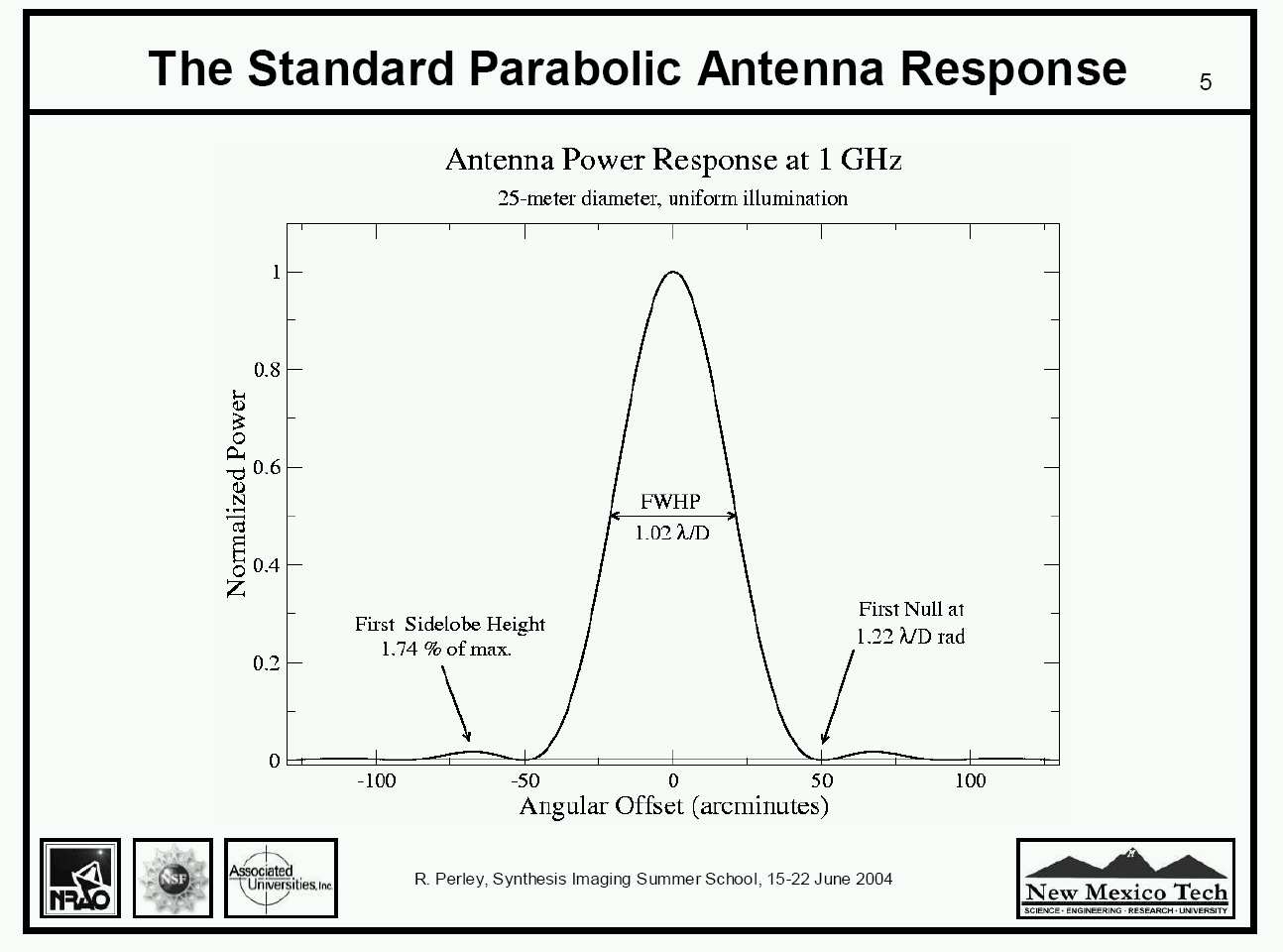

The focusing ability of a lens or mirror type antenna is directly related to its width in wavelengths of the radar wave. The wider the antenna is in wavelengths the smaller the angle of the beam that contains 50% of the radiated energy. The smaller the angle of the beam, the farther the radar can see the target and the more precisely the angle of the target can be known. Nike tracking radars had an effective antenna width of about 150 wavelengths. (The antennas were actually physically a little larger, but there are edge effects which decrease the focusing effect of the edge areas.) 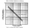
from "Early Fire-Control Radars for Naval Vessels", "Bell System Technical Journal", Jan 1946 http://www.alcatel-lucent.com/bstj/vol25-1946/articles/bstj25-1-1.pdf 35 MByte
Beam width - A rough (somewhat optimistic) formula for the beam width is
BeamWidthInDegrees = 57 * WaveLength / AntennaDiameterRadar Range
where WaveLength and AntennaDiameter are in the same units.
A small (narrow) beam width in an acquisition antenna is a "good thing", giving more more radar energy on the target (better range), and better target angle determination. An odd thing about an acquisition antenna is that you often want to see all the targets at an azimuth regardless of target elevation (lets not worry about directly over head - it would be too late if a target got there). So frequently acquisition antennas are wider than tall, giving a narrower azimuth beam width than elevation band width. This compromise permits better detection of targets regardless of their altitude.Nike tracking radars focused more than 50% of the radar pulse into a beam less than 1 degree wide, both horizontally and vertically. The acquisition radar beam was about 1 degree wide horizontally, but spread out vertically into a fan shape to see aircraft both near the horizon and also higher up.
This Bell System Technical Journal link discusses the Metalic Delay Lens used in Nike Ajax - 1948
to any echoing object is measured by determining the delay between the transmitted pulse and the echo. The speed of a radar wave in air is about 300 meters per microsecond. (It varies very little with normal ranges of altitude and weather.) The round trip time for a radar pulse from transmitter to echo object to receiver is about 150 meters (164 yards). With electronics, measurement of the echo time to with in 5 meters is no technical challenge.One Antenna, and the T-R Tube
is used for both transmitting and receiving. This is actually rather tricky, as the transmitter sends a pulse of energy to the antenna sufficient to cook or spark most receiving components, then with in a few micro seconds, the transmitter must be electrically disconnected from the antenna and the receiver connected.The MagnetronThis is microsecond switching function is performed in the radar "wave guide" by a "duplexer" circuit usually using a "TR" tube (transmit/receive tube). Basically, the powerful radar pulse causes an arc in the TR tube (in the wave guide), and the arc, being a conductor reflects most the pulse away from the receiver connection, keeping the pulse from the delicate receiver components.
The following images are from the "Bell System Technical Journal", ( BSTJ )
"The Gas-Discharge Transmit-Receive Switch"
http://bstj.bell-labs.com/BSTJ/images/Vol25/bstj25-1-48.pdf
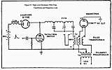
This is the basic single antenna pulse radar circuit used from about 1942 until the present day. 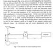
This tube was current in 1942. The tube the Nike Ajax Tracking Radars (developed about 8 years later) was a metal box about 1 inch x 1 inch x 0.5 inch with a flat quartz window on one 1 x 0.5 inch face. We were told that the inside of the tube was radioactive ( maybe tridium? ) and don't break them open. We were told that during the magnetron pulse, and arc or plasma formed on the window reflecting the power away from the sensitive receiving diode. 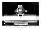
Microwave Oven Magnetrons
Please note: the following history was written in 1999, and was the best widely available information.
Now, with Wikipedia, much more history of the magnetron is widely available.
Currently, 2016, "radartutorial.eu" seems a more complete, compact start.
Also see, investigations into magnetron like devices, from "Gdessornes" .Before 1939, radar waves were created using rather standard vacuum tubes. The tube shapes were changed to permit shorter wires (higher frequencies) but even the best technology was limited to pulses of about 2,000 watts at about 700 megahertz (700,000,000 waves per second).
There was great desire to get higher frequency (for tighter beams with smaller antennas) and higher power (for longer range).
A tiny bit of the intense struggle.
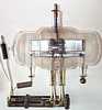
Images to the left are Eimac VT158 from http://www.r-type.org/exhib/aac0090.htm used in the AN/TPS-3 (SCR-602), image to the right
"The VT-158 is an unusual American transmitting triode. It was designed for pulse operation at 500 MHz, and would produce 200 kW pulses. It was used in the TPS3 radar. The envelope contains four valves in two pairs. The anodes are connected together but brought out to twin connections. Tuned lines were fitted to the anode connections, but these have been removed from our specimen. The inset picture shows the bright helical filament in one cavity. Surrounding the filament is a dull grey wire cage grid. The anode is finned and substantial. The wide glass tube envelope is 87 mm in diameter and, excluding the base pins, is 200 mm tall."
In 1940, the British developed a remarkably simple sounding method of generating an intense pulse of radar waves. This was the multi-cavity magnetron The arrival of the secret working British prototype magnetron into the U.S. caused great hope and excitement. The British prototype could deliver 10,000 watt pulses at 3,000 megahertz. This was 5 times the power (great!) at 4 times the frequency (wonderful!) of the best current technology. And the current technology seemed just about at its maximum (the components and systems had been pushed and tweaked extensively). And the newly developed magnetron from the British was just a research prototype - there could be room for big improvements.
This was a stunning "breakthrough". See "A History of Engineering and Science in the Bell System: National Service in War and Peace (1925-1975)" for further details.
This research type magnetron was delivered to the U.S. in October 1940 and demonstrated at Bell Telephone Labs. The British prototype was certainly improved in the U.S. for much higher power, manufacturability, stability, frequency adjustability and range, and other factors, but the impact of this basic invention on the successful Allied radar development was very great. It turns out that the mass manufacture of high performance magnetrons is much more tricky than first imagined. There were whole new worlds of large glass/metal seals, permanent high vacuum evacuation of machined metal castings, manufacturing tolerance of the cavity size and shape, cathode resistance to back bombardment, etc to be solved. Bell Labs and Western Electric made more than 100,000 magnetrons of various frequencies and powers for World War II.
This is another serious history local copy - about 1 megabyte .pdf - and an interview with Edward M Purcell
This "tube" helped guide the British fighter planes in the "Battle of Britain" bombings and gave the British (and the Americans) an advantage in the radar race until the Germans also developed one (from a downed British bomber?).
The 3,000 megahertz magnetron perfected from the British prototype had a very large (30 pound, 14 kg) magnet with a metal and glass "tube" about the size of a hockey puck (small can of tuna). (Higher frequency, shorter wavelength magnetrons and magnets are smaller and lighter.) It had a peak power of 1,000,000 watts (an improvement by a factor of 100). It was rugged and reliable.
The above is a diagram of a magnetron (without output loop)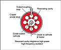
Wikipedia Cavity Magnetron, not available when much of this was written.
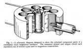
from Fig. 1, BSTJ, April, 1946 106 MBytesNotes : Not shown are two contacts for the cathode. These allow for cathode heater current (remember vacuum tubes had a hot part called the cathode to "boil off" electrons into the vacuum?). A special 5ish volt transformer was used which permitted the whole cathode to be at 18,000 volts during the short (about 1 microsecond) time the magnetron "fired". "Interesting" currents (about 100 amps) of the high voltage were required to generate 1,000,000 watts of peak power. To get such currents emitted into the vacuum from the required small cathode, a coated cathode was used. This coating could be damaged more easily than the normal thoriated tungsten used in the usual high power tubes. The magnet and copper anode stayed at "ground" (zero volts).
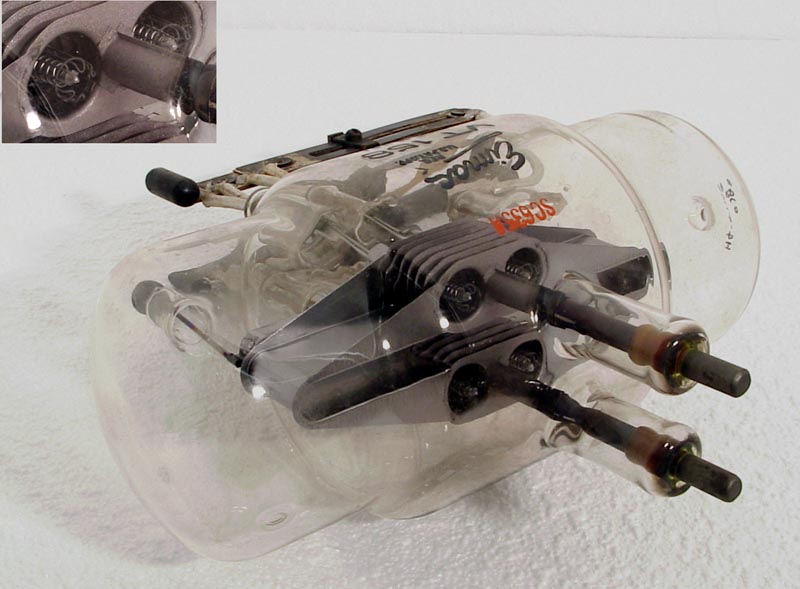
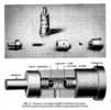
Nike LOPAR Acquisition radar used the 5795 magnetron made by Western Electric
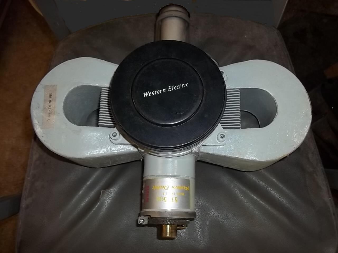
This is the cathode end with the big glass insiulator to isolate the high voltage pulses. The metal rings at the end of the glass are for the filiment and cathode connections. 
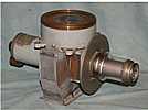
The magnetron is tunable via the gearing, to about +-10 % nominal frequency. An automatic frequency control circuit from the wave guide tracked the receiver to the transmitted frequency. Nike X-Band Magnetron, for TTR and MTR - Photo by Greg Brown
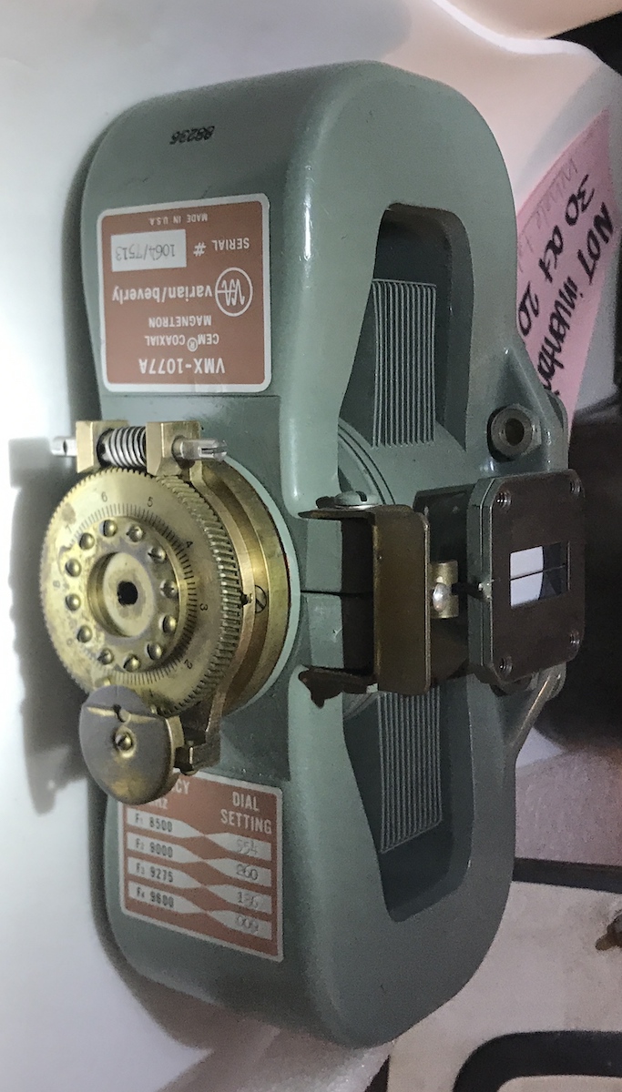
DIAL SETTING FREQUENCY MHZ 554 F1 8500 260 F2 9000 136 F3 9275 009 F4 9600 Apparently the Brits were not the first to play with slotted magnetrons, but we heard of their efforts first - and history gets biased -
There were many interesting effects in the magnetrons (as in most of the other radar components). For instance, after the cathode was heated by the filament current, and the magnetron was pulsed with the high voltage pulses, there were so many electrons that would gain energy then come crashing back to the cathode that the cathode would over heat unless the cathode heater current was reduce or eliminated.
For a detailed description of how a radar magnetron works, see Magnetrons.
Here is a 30 minute Air Force movie of magnetron maintenance.
And getting the power out of a magnetron, along with
- tuning the output over a 10% range
- arcing
- design variations such as "Amplitron"
can be "interesting".
The Modulator
You may note that your home microwave oven is "instant on" - no waiting for minutes for the cathode temperature to stabilize -
This type of magnetron uses an undesired effect in the hot cathode (high powered) magnetrons called "Secondary Emission" which adds undesired heat to the cathodes of hot cathode magnetrons. (While operating hot cathode magnetrons, the filament current is reduced to prevent overheating the cathode.)This paper and this web page discusses cold cathode secondary emission used in your "instant on" microwave oven. (The voltage in your microwave is about 300 volts :-))
- A special circuit (modulator) would suddenly put a high voltage (and high current) across the magnetron and out would come powerful radar waves. In the LOPAR acquisition radar, the modulator put about 18,000 volts at 100 amps for 1 microsecond through the hockey puck sized "tube" of the magnetron. The magnetron would put out about 1,000,000 watts of radar waves during this microsecond. This is repeated 400 times per second. - a nice trick - do that with your flashlight switch ;-))The Nike LOPAR modulator thyratron was the 5948A
Mechanical
SchematicThe most noticeable component of the LOPAR modulator was the hydrogen thyratron tube. This tube tube was about 12 inches tall and about 5 inches in diameter. This was the tube that switched the 18,000 volt 100 amp current mentioned above on very quickly, about 0.05 microsecond. The hydrogen gas in this big tube glowed violet when it was working. A "delay line" circuit was used to help limit the length of the pulse.
This is why hydrogen is used in radar modulator tubes, rather than mercury.
from https://aobauer.home.xs4all.nl/Evolution%20of%20Hydrogen%20Thyratron.pdf
Quick summery - faster de-ionization time permits higher "Pulse Repetition Frequency" (PRF).
ElectricalThis modulator tube took about 15 minutes to warm up properly. (Every thing else in the Nike system warmed up adequately in 5 minutes or less.) A 15 minute timer prevented the tube from being used during this warm up period. (There was a timer over-ride circuit so that it could be used sooner in a "battle emergency".) One night during the beginning of a routine alert, the captain got impatient waiting for this timer and activated the over-ride switch after about 10 minutes. The tube seemed to work just fine, the radar worked fine, nothing bad seemed to happen.
Quick notes:
- "PFN" below is "Pulse Forming Network" which helps provide a, squarish pulse to the bifilar transformer :-)) The squarish pulse helps keep the magnatron near a center frequency during a pulse ( within the band pass of the receiving IF amplifiers.) In the conventional magnetron, operating under a condition of space-charge-limited emission, an increase in anode voltage produces an increase in anode current. This is accompanied by a small shift in frequency termed "pushing."
- The chock "Lch" and Charging Diode for a convenient voltage doubling circuit.
This diagram seems wrong, the voltage on the thyratron and pulse transformer should be 12,000 volts. The charging diode, Lch, and action of the pulse forming network provides a voltage doubling function, giving 12,000 volts on the pulse transformer and onto the magnetron.- The schematic to the right is from an unidentified manual.
Pulse transformer windings.
- The dots you see on the transformer windings (T1) in Figure 63 indicate points having the same polarity. Thus, if one dot represents a negative polarity, then all the dots are negative. Notice the secondary, connected to the magnetron filament. The secondary is bifilar, that is, the two secondary windings are wound side by side on the core. Wound in this manner, the secondary has exactly the same voltage induced into each winding.
The Nike tracking radars had physically smaller (higher frequency) components with about 1/4 of the peak power (250,000 watts) and 1/5 the pulse width (0.18 microseconds).
Bill Shaw reports that the NIKE Hercules Tracking Radars used a different pulse modulator. Not a thyratron but a huge vacuum tube, the Machlett 6544 data sheet -

Here are 2 from the Nike radars that were duds. Changed many of them but normally just junked them when bad but saved two and made lamps from them. They are Machlett 6544 tubes from the TTR and MTR radars. These are 14 lbs apiece Biggest tube I ever saw and changed was the huge 15MW Klystron in the HIPAR mounted vertically and cooled by ethelene glycol
Bill ShawFor more on modulators, see the technical manual of a similar modulator Modulator and transmitter of the AN/TPS-1G ST-44-188-3G from Chuck Zellers - 2.5 megabytes
the Klystron another microwave source
In 1937, just before World War II, a device called a klystron was developed by the Varian brothers in California. In 1939 a handy form of "klystron" called a reflex klystron was developed in England by Robert Sutton.During World War II, the klystrons were primarily the reflex type and were used primarily as low power (milliwatt) oscillators in test equipment and radar and microwave receivers.
By the 1950's, there was a considerable demand for high power (kilowatt average power) microwaves, but with more precise control than could be generated by magnetrons. The customers were communications, medicine, science including particle accelerators, and radar. The Varian brothers, with the patents and the skills, did very well. Soon klystrons with average powers of 50 kilowatts and peak powers of 50 megawatts were available. To achieve the high current electron beam densities at these powers, powerful magnets (usually electromagnets) surround the tube. To get the most power from each electron in the beam, very high (100,000) voltages are typical.
These powers were impractical with magnetrons. The klystrons could deliver both the higher powers and also could amplify low level precise signals to these high powers. The klystrons were much larger (up to 2 meters long) and with their magnetic solenoids quite heavy (500 kilograms) and more expensive ($50,000), and more troublesome to keep running (required vacuum pumps) but they could be much more powerful and precise than magnetrons.
Power klystrons, such as described above have power gains (output signal/input signal) of over 10,000. As a comparison, typical power transistor in your stereo has a power gain of 20.
The Nike HIPAR radar transmitter used a
powerful klystron. 57 K Bytes. Image from Rolf Goerigk This one is about 5 feet tall 18 inches in diameter (including a focusing magnet - solenoid), and could output 10.4 megawatts peak pulse power - average power was 26 kilowatts. To help get that peak pulse power, 210,000 volts were used. This voltage gives much more powerful and numerous X-rays than your doctor's office machine - yes - the tube was surrounded by a lead shield.
The cooling system included 60 gallons of mixture of ethylene glycol and water (anti-freeze).
Yes - Lead Shield - There was a report that some technicians on the DEW line were tying to trouble-shoot a similar BIG klystron - and decided to remove the lead shielding for a while - If I remember the report correctly :-(( two of the technicians died with in two weeks of radiation "poisoning". I can't find the reference :-(( This class of tube does not sit happily in a glass tube and run unattended for years. The vacuum needed to be very high, and the klystron needed to be attached to a very good vacuum pump while in operation.
Because of possible rapid and precise changes of the frequency, amplitude, and phase of the output radar waves, very interesting receiver options are available to increase receiver efficiency (detect less reflective or further targets) and also to help suppress the effects of jamming (ECM).
Reflex klystrons were used as local low power ( 0.1 watt) microwave oscillators in many of the Nike radar receivers and test instruments.
Gary Evans asked if a "twystron" was used in the Nike system. I replied that I didn't think so - what is a "twystron"?
... AN/FSS-7 had a hybrid TWT/Klystron output device. The twystron was a big unit. stood about 4 foot tall , waveguide out direct to antenna system. Really seemed big for a freq in the 1-2 Gig range as I recall. Had a watercooling system. Ran a peak output of 4 Megs, but only a average of 7KW or so. (Short duty cycle - 20 microseconds transmit / 850 NM listen). Had a gigantic focus magnet around it (1000# or so) I seem to recall the Raytheon name on the side of the box it shipped in.
Wave guides (some times called "radar plumbing") are simple and complex at the same time. Radio waves can travel inside of a conductive (copper) pipe as long as the inside circumference of the pipe is longer than 1/2 of the wavelength of the radio wave. (Low frequency radars require larger wave guides.)
Radar waves can go through the convenient coaxial cables (similar to your cable TV lines). However there are several problems:
- Losses (attenuation) increase with frequency, and can get impractical at higher radar frequencies.
- Isolation between cables can get to be a problem.
- Peak power (related to maximum voltage) is quite limited.
Wave guides greatly reduce the above limitations and provide some interesting advantages:
- The greater conductivity of the greater surface of copper greatly reduces the resistivity and the air (or vacuum) in the cavity is a much less lossy dielectric than most available in coax cable.
- The thick solid walls are almost perfect isolators, preventing leakage into and out of the waveguide.
- The greater distance from wall to wall allows much higher voltages (and peak power).
- Various rotating, adding and subtracting tricks are much easier with wave guides.
For the above reasons, wave guides are very popular in radar units, even though they are more expensive and bulky and much less physically flexible. The cross section for the LOPAR antenna is about 1.5 inches by 3 inches (about 3.5 cm by 7 cm). The cross section for the X band tracking antennas is about 0.5 inches by 1 inches (about 13mm by 26mm). To provide better control of the various internal transmission modes, wave guides are usually constructed with a rectangular cross section. This limits some of the undesirable electrical modes possible in circular cross section wave guides.
All of the radars in the Nike system used wave guides. Almost all of the radars you have ever seen use wave guides. (The little radar receivers used to detect police speed radar "guns" use other methods.)
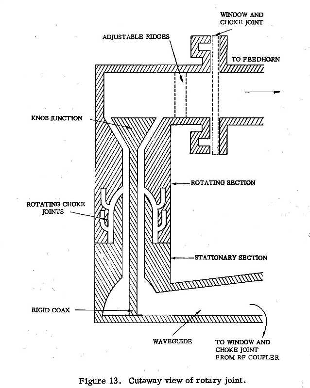
Most large acquisition radars have the magnetron in a fixed location. How do you get the radar waves from the fixed wave guide to the rotating wave guide if the radar "dish" is going round and round, and the magnetron is sitting in a fixed place?
A very practical question. The answer is a rotating microwave joint. At the center of rotation, the rectangular wave guide merges into a circular wave guide. The circular wave guide forms the center of the rotation. There is a trick used so that the copper of the rotating part does not need to touch the copper of the fixed part. Up in the rotating part of the antenna, the circular waveguide converts again to a rectangular wave guide and on to the feed horn (the part that lets the radar waves out into the air - or back again into the wave guide).For various reasons, Nike tracking radars have the magnetrons and receivers in the rotating part of the antenna. Later when we discuss "How The Tracking Radar Points at an Object", these rectangular wave guides will split the energy from the feed horns, rotate the waves, combine the waves in a subtractive way, do some more electronic tricks, and get antenna pointing error information. Just like magic.
A 25 minute Air Force movie about wave guides.
Return to beginning of Nike Radars
Radar receivers are very similar to your usual TV receiver, and in many ways simpler because we don't have to play such interesting games processing the audio and color video. So we will just consider the TV "front end" through to the beginning of the audio and video (throwing out about 3/4 of the TV electronics.
All of the components are similar in function, and most are almost interchangeable with a radar set. The big difference is the front end where the incoming frequency is much higher. We will see that we quickly reduce the frequency to TV IF (intermediate frequency) and any TV repair person can take it from there.
Component
Nametypical
TVtypical
radar...
CommentTuned Circuit 60-500MHz 3000-16,000MHz reduce undesired frequencies Mixer a tube
or transistora crystal output difference between signal and oscillator Oscillator 87-527MHz 3030-16,030MHz produce "beat frequency" for mixer, could be a klystron Auto Freq Control same same (AFC) controls frequency of oscillator AFC gate tracks sync pulse tracks magnetron pulse track only transmitted signal IF strip 27 MHz . increase signal to desired voltage using single frequency . . 30 MHz (acquisition radar) this lower frequency reduces noise . . 60 MHz (tracking radar) higher frequency to increase range resolution Auto Gain Control same same control gain of IF strip Gain Gate tracks sync pulse tracks target control gain of desired object Detector same same convert intermediate freq to video More correctly, military radar receivers are somewhat different from your TV in internal details to increase ruggedness, testability, maintainability, and to reduce the effects of various forms of enemy jamming. The field is large and complex and is beyond our scope here.
HOWEVER - a related acquisition pulse radar receiver AN/TPS-1G Receiver System ST-44-188-4G from Chuck Zellers - 2.08 megabytes is on-line at this web site. :-))
Since the radar frequency is about 1/3 that of the Nike LOPAR acquisition radar, some of the technology is slightly different - such asbut the cross-training is simple and quick - such what/where are the components and where are the interlocks. A bit like the differences in repairing two different brands of automobiles or washing machines.
- local oscillator is a different tube
- co-axial cables are used more in the AN/TPS-1G than wave guides
Return to beginning of Nike Radars
Most radio receivers (including your AM/FM, TV, cellular phone, and radar set) convert the received radio waves to a fixed frequency for amplification. This conversion is actually much simpler than trying to tune about 5 high gain stages through the desired frequency range. (See Wikipedia for a discussion on Superheterodyne receiver.) This group of about 5 high gain amplifier stages is formally called the Intermediate Frequency Amplifier or more commonly called the IF Amplifier. This technique saves many microwave amplifier design, fabrication, and adjustment headaches.
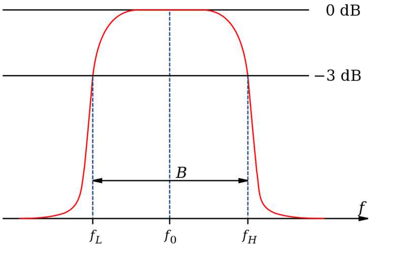
A small note: IF Amplifiers are usually "stagger tuned" to provide rather even amplification over a limited range of frequencies "band pass" to allow rather sharp pulse edges to be passed. This image and further discussion can be found at Wikipedia 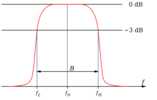
The usual frequency in most radar sets for the IF Amplifier is about is about 40 megahertz (give or take 20 megahertz). To convert an example input radar signal of say 5,000 megahertz down to say 40 megahertz for the IF Amplifier you generate a signal 40 megahertz away from the input radar signal (in this case 5,040 megahertz is fine). The unit to make this extra frequency is called the "local oscillator".
Put this "local oscillator" signal, and the input radar signal together into a "mixer" (which contains a non-linear element). The output of the mixer will contain all of the input frequencies plus the sum of the input frequencies (10,040 megahertz, which is not used) and the difference of the input frequencies (40 megahertz) which is amplified by the IF Amplifier.
The local oscillator at radar frequencies is usually a little reflex klystron .
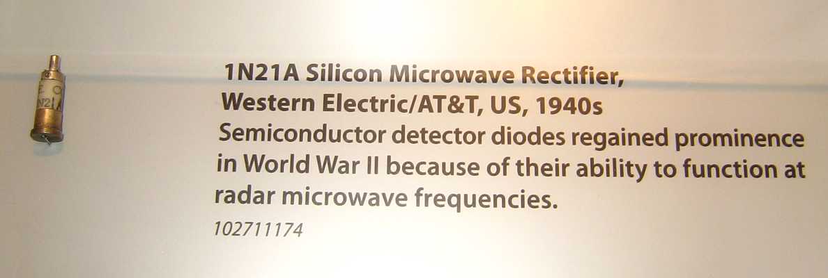
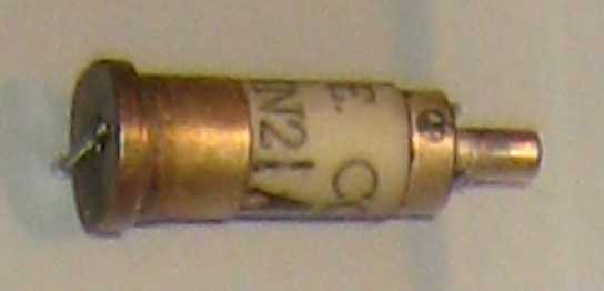
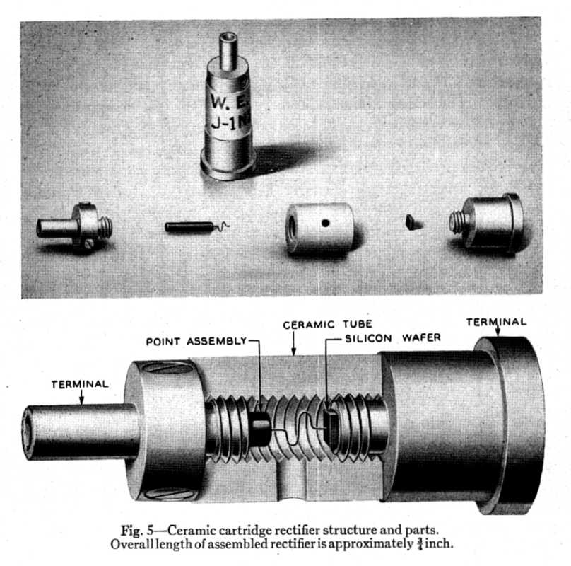
The mixer can be a radio tube below about 1,000 megahertz, but above this frequency the radio tube is too inefficient and noisy. A "crystal" mixer was used in almost all of the radar sets during the 1940s and 1950s, (and is still in common use today in many commercial radar sets). (During the 1960s, a "traveling wave" tube was developed which could be made to have even lower noise than the crystal mixer. This is used in some demanding military, space, and research receivers, and was used in the Nike HIPAR radar receiver.) (For a 1942 paper on "Theory of High Frequency Rectification by Silicon Crystals" (written before the invention of the transistor) click here. 725 KBytes - spotted by R. Tim Coslet. ) The 1N21 is rated NF 16.4dB at 3GHz, frequency of the LOPAR acquisition radar
The 1N23 is rated NF 17.1dB at 9.37GHz, frequency of the MTR and TTR tracking radars
Identical form factors.
Nike Radars used similar crystal mixers
Image from http://bstj.bell-labs.com/BSTJ/images/Vol26/bstj26-1-1.pdfSo - in 1939 the invention of the magnetron permitted reasonable radar above 1,000 megahertz, and reliable, rugged crystal mixers were developed as low noise mixers to handle this higher frequency range. The research at Bell Labs that helped create those crystal mixers led directly to the invention by Bell Labs of the transistor a few years after the war and to the continuing semiconductor revolution and to your computer.
We adjusted the local oscillator power going into the crystal to give a crystal current of about 2 milliamperes. Too little power gave lower mixer efficiency, too much power gave more local oscillator generated noise.
We have described many of the interesting radar components above. If we could visit a radar component supermarket (close out sale today), we could select components and build our own radar. Actually millions of people assemble components for their IBM clone computers and survive about the same complexity. There is a big difference in size, weight, voltage and powerful microwave radiation hazard. The general schematic would be:
The components and their uses are:
Component Comments Start_Pulse_Generator One pulse a few microseconds before each radar pulse Power Supply 18,000 volts, otherwise a bit boring Modulator Sends a powerful 1 micro second pulse to the magnetron Magnetron Makes powerful radar waves (for 1 micro second) TR Tube Keeps most of powerful radar waves out of the receiver Receiver Amplifies the returned radar waves, giving video Display Tube Shows the return radar waves/video to the operator (PPI) (A scope) Tracking Unit Helps follow the selected signal in range, azimuth, elevation I must apologize to designers of military radars who add many small enhancements to reduce the effects of enemy jamming (and accidental friendly jamming). These enhancements may include:
- funny looking fins to reduce antenna side lobes
- facilities to easy rapidly change radar frequencies
- facilities to quickly change number of radar pulses per second or skip pulses
- changes in receiver details to counter overloads
- changes in receiver details to automatically/manually reduce sensitivity to certain patterns of jamming,
- and this list could go on for a number of pages
And the above list is for magnetron oriented pulse radars. This is the usual radar for private use, boats and ships, etc. The klystron based radars are not so common outside of military and research (such as imaging asteroids) use. Anti-jamming using these radars can be even more can be even more exotic. Or you can WOW your neighbors and buy major Nike system components, see How to get Nike Parts? .
Acquisition Radar (the wide eyes)
The Acquisition Radar is a most interesting looking radar. It is large and has motion, going round and round. It is often called a "surveillance" radar, providing the slant range and azimuth (direction) of all the radar visible objects in the area 5 to 10 times a minute.
A tiny bit of radar history
Before the Brits let the US in on their secret radar transmitter breakthrough, the Cavity Magnetron, the Americans were making radar sets the conventional way - with specially designed rather high frequency, rather high power triodes.
While I was at Chicago (1954) we had (for a few months) a very senior (like going to be retired at that rank) 2nd Lt. The poor fellow likely would have made an adequate Warrant Officer - but a rather hopeless commissioned officer. He was really a Dilbert type nerd, fine technically, but ... :-(( He said that early in WWII, he had tried to tune acquisition radar transmitters that were pre-magnetron. The final amplifier was a ring of special triodes, set in a physical circle. Tuning that big parallel arrangement was difficult and time consuming.) Our magnetrons (1954) were basically "plug and play" ;-))
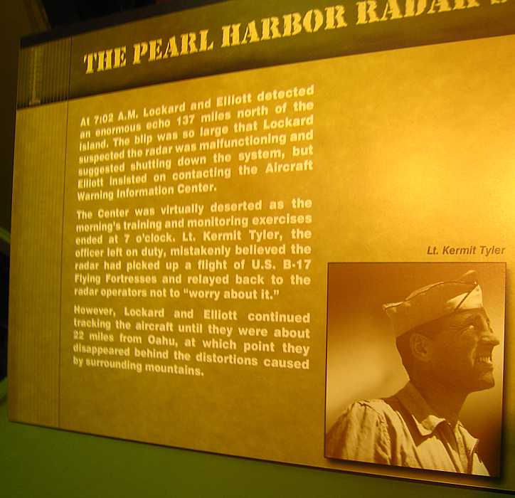
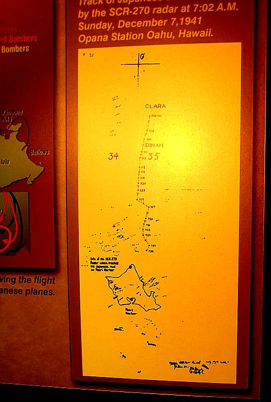
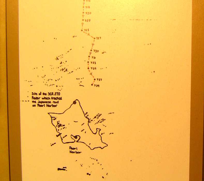
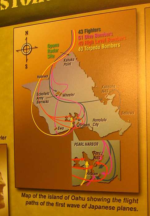
In any case,- the Army had just installed an SCR 270 type radar on a Hawaiian mountain, :-)) - looking west, on Sunday, December 7, 1941 :-)) - The operators detected and tracked a large flight of inbound airplanes, :-)) - which later turned out to be a Japanese attack force :-(( - They reported their find to HQ, :-)) - which did not recognize the threat :-(( Here is a display at the National Electronics Museum near Ft. Meade, MD. A great place to visit! :-))
Intro 
Track over the ocean 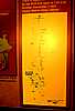
enlarged 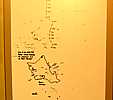
over the island 
Just for fun - some REALLY huge radar antennas - BMEWS
Ballistic Missile Early Warning System had really HUGE antennas -- each 165 feet (50 m) tall and 400 feet (120 m) wide, using 425 MHz frequency.
Over the horizon radar - "typically hundreds to thousands of kilometres, beyond the radar horizon,"Usually surveillance radars have a longer wavelength than the tracking radars, as minimum beam width is less important. In the case of Nike, the LOPAR surveillance radar had a wave length of 10 centimeters (about 3,000 megahertz). (The Nike tracking radars had a wavelength of 3 centimeters or less.)
Charles D. Carter asked the question
"What is the difference between a HIPAR, LOPAR and ABAR?"
from Chuck Zellers Aug. 2009, via Charles D. Carter
LOPAR is the low power acquisition radar used in every Nike Ajax/Hercules site. LOPAR was used to "acquire" a target. ABAR is the "Alternate Battery Acquisition Radar" (AN/FPS-75) is the military designation, which was used on many Nike sites as a low cost alternative to HIPAR. HIPAR or "high power" Alternate Battery Acquisition Radar" as a high power (transmitter). Both ABAR and HIPAR were used as an acquisition radar that passed targets, typically ones that LOPAR could not acquire because of distance, etc. The HIPAR surveillance radar - ( AN/MPQ-43 ) had a wave length of 23 centimeters (L-band, about 1,300 megahertz) and an effective range against large high-flying non-stealth aircraft of about 200 miles. The HIPAR radar had a large control building. There was very sophisticated pulse generation, and multi-channel receivers with unique moving target indicators (MTI) and great deal of anti-jamming capability. It was made by General Electric.
See names and faces here
Doyle Piland says
"The best I can find is that the Fixed HIPAR was AN/MPQ-43 and the mobile HIPAR was AN/MPQ-44."
Also
http://www.mobileradar.org/radar_descptn_2.html notes MPQ-44 ñ Notes: A mobile version of the HIPAR radar (AN/MPQ-44) was deployed in 1967. It is mounted on five trailers and includes all of the necessary power generating equipment to operate the entire Nike Hercules fire control system. The radar is designed to be used in the ATBM or EFS configuration and, like the fixed-site HIPAR, the mobile system also uses the presentation system of the Nike Hercules system. (Ref: US Army Air Defense Digest, 1972)
Thomas Page notes
"... except the 'M' in AN/MPQ designates "mobile" ... "
Ed Thelen says "Glad I was just a techie - leaving the complexity of naming things to others ;-))"

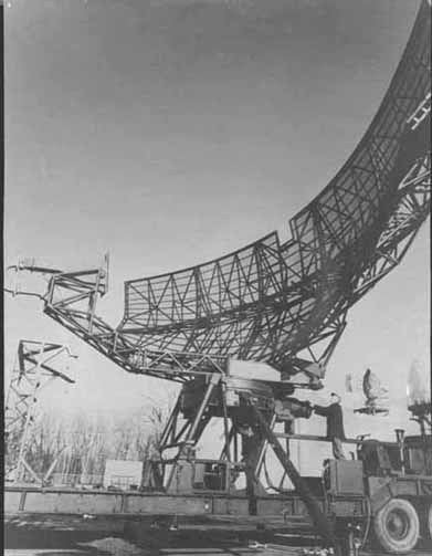
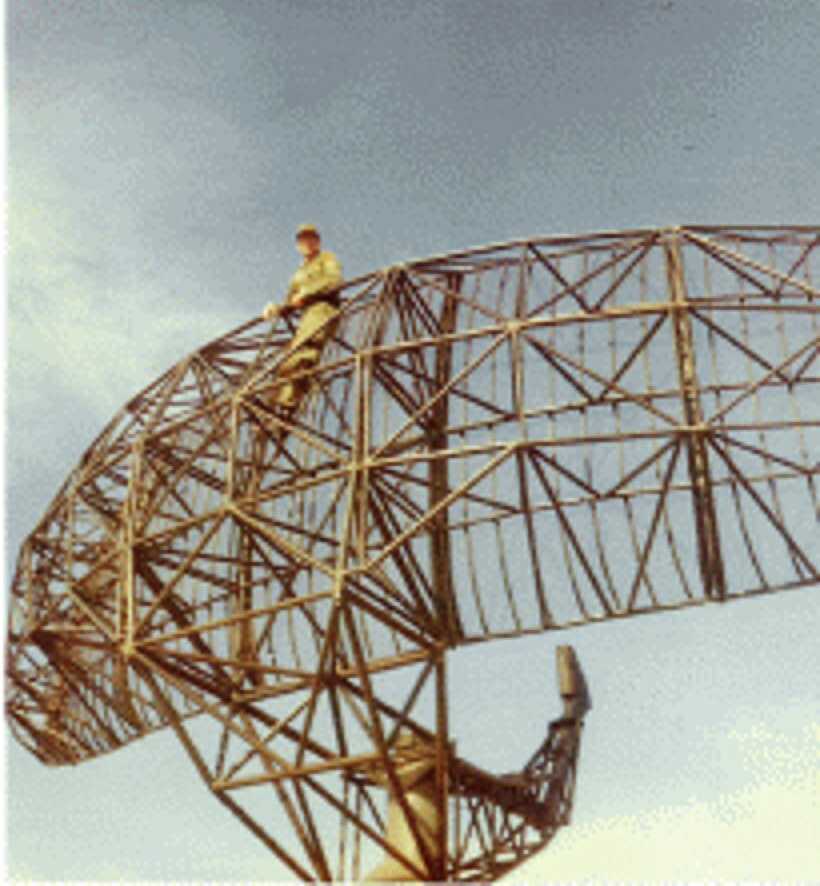
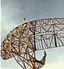
A Nike HIPAR radar antenna with out protective radome, image is 74 K Bytes
(Photo credit - page 303 "Jane's Radar and Electronic Warfare Systems", 18th edition.) There is information that this picture does not include: 1) an anti-jamming antenna at the top of the main antenna, 2) two small antennas on each side, 3) an IFF antenna.
A Nike HIPAR FAN radar antenna , image is 53 K bytes.
(Photo credit Rolf Goerigk
A Nike HIPAR radar antenna with protective radome, image is 60 K Bytes
(Photo credit - adapted from Bill Benson , benson@efdata.com)
Note that the HIPAR antenna is high on a pedestal. There are 2 main reasons,
1) have the high power beam safely above any near by personnel
2) to gain a little range over the curvature of the earth.

Drawing of HIPAR Station image is 71 K Bytes
Image from Rolf GoerigkFrom Rolf Goerigk, Specification for the HIPAR include:
Polarization horizontal Antenna Gain CSC2 antenna = 34.8 dB = 3020 ("CSC2" stands for co-secant squared, a vertical pattern optimized for aircraft detection at low and high altitudes and ranges)
FAN antenna = 29 dB = 790Beamwidth 1.2 deg Azimuth at 3 dB
1.3 to 7.1 in elevation
FAN 1.35 deg at 3 dBVertical Coverage 0 to 60 deg., 46 km height, 425 km length Antenna Speed 6.6 and 10 RPM (Revolutions Per Minute) Azimuth Accuracy > 0.25 deg. Noise max. 6.5 dB (1005 deg. Kelvin) Reflector Dimensions height 6.3 m (20.6 ft.), width 13.11 m (43.0 ft.), 82.6 sq. m (900.9 sq. ft.) - BIG Pulse Width 6 microseconds RF Freq Range 1350 - 1450 MHz (10 channels) RF Power: nominal: 10.4 MW / 26 kW average For a more detailed description of HIPAR, see Lesson 3. HIPAR Acquisition Radar - 1.7 megabytes
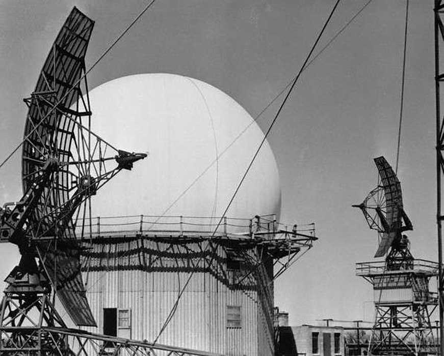
The "antenna" - the big reflecting structure of the usual acquisition radar is much wider than tall. This gives a radar pattern that is narrow horizontally and wide vertically. This is desirable when looking for aircraft (or ships) in the area. This pattern gives good information about range and the azimuth angle (to about 1 degree) but gives little information about the elevation angle. Range times the sine of the elevation angle gives the elevation of the target - often very useful. So, near large defensive acquisition radar antennas, were frequently placed "Height Finding" radars which provided accurate elevation angles (to about 1 degree). This enabled the defenders to know the height of the target aircraft to better evaluate the threat and better direct defensive aircraft to the target.
The unusual looking up/down radars near the dome are height finding radars. They can point in any horizontal direction, then nods up and down to find the strongest elevation angle of the target at the proper range.
this text and image is from HTTP://www.radomes.org/museum/equip/radarequip.php?link=fps-6.html
The AN/FPS-6 radar was introduced into service in the late 1950s and served as the principal height-finder radar for the United States for several decades thereafter. Built by General Electric, the S-band radar radiated at a frequency of 2700 to 2900 MHz. Between 1953 and 1960, 450 units of the AN/FPS-6 and the mobile AN/MPS-14 version were produced.The HIPAR radar was very expensive, and was only used at selected Hercules sites. The other Hercules sites had "Alternate Battery Acquisition Radar"(ABAR) radar which was not so sophisticated, not so long range, and not so expensive. There were three models called "ABAR", the models were identified as AN/FPS-69, 71, and 75.
AN/FPS-71
A catalog description of the AN/FPS-71 included the following phrases:
- 40 ft. reflector
- Frequency: 1220 to 1350 mHz
- Range, Max: 200 naut. mi, Min: 300 yd.
- Peak Power Output: 5 Mw, Pulse Width: 2 us, Pulse Rate: 325 to 400 pps.
- Peak Power Handling Capacity: 2 megw at .001 duty cycle
- Horizontal Beam Width: 1.4 deg. at half power points
- Vertical Beam Width: 6.2 deg. at half power points
- Special Features: Antijamming circuit that limits width of echo pulse that receiver will pass.
https://www.radartutorial.eu/19.kartei/11.ancient3/karte095.en.html has more information.
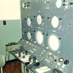
Likely to be the display system for an ABAR AN/FPS-71.
From Al Kellogg via Greg Brown
Peter DeMarco wrote about the AN/FPS-75
The ABAR we had in Alaska was the AN/FPS-75. I can't compare it to HIPAR but it had a range of about 200 miles and the ECCM equipment on it was very sophisticated. There were 6 different radar presentations I could view at the same time. Lots of buttons and lights. Chuck Zellers wrote about the generations leading to the AN/FPS-75 ABAR radar
I had written about lots of AN/TPS-1D (Tipsy Dogs) at Ft Bliss in 1954.May, 2008, Chuck adds ;-))
There a few differences between the AN/TPS-1G and the AN/FPS-36. The large schematics and one of the ST-44-188 manuals describe such differences. [See manuals.] The family of radars these systems belong to include the AN/TPS-1D (called tipsy dog). The AN/FPS-36 is a fixed radar system whereas the TPS series are transportable, hence the TPS designator. The FPS is the "fixed," non transportable designator. The FPS-36 has a much larger antenna (40'x11'), a pulse generator to generate a lower PRF, pulse repetition frequency. This allows the max range for the -36 to 200 nautical miles as opposed to the 160 NM for the AN/TPS-1G. The 36 receiver is also enhanced with a better signal to noise ratio. The receiver/transmitter and azimuth-range indicator are changed to allow the 200 NM range. The -36 uses a waveguide as opposed to the large coaxial cable used by the 1G.
The AN/FPS-75 is an AN/FPS/36 that is interfaced with the LOPAR PPI to allow ABAR video sweep presentation on the Acq PPI.
Me circa 1964 on a AN/FPS 75 (ABAR)Many of the components from each system are interchangeable.
Googling "5J26" which is the magnetron used in the AN/TPS-1D/G and AN/FPS-36/75 ABAR radars provides additional info on the subject. Interesting and you can even purchase a 5J25 for a cool $3500.00!
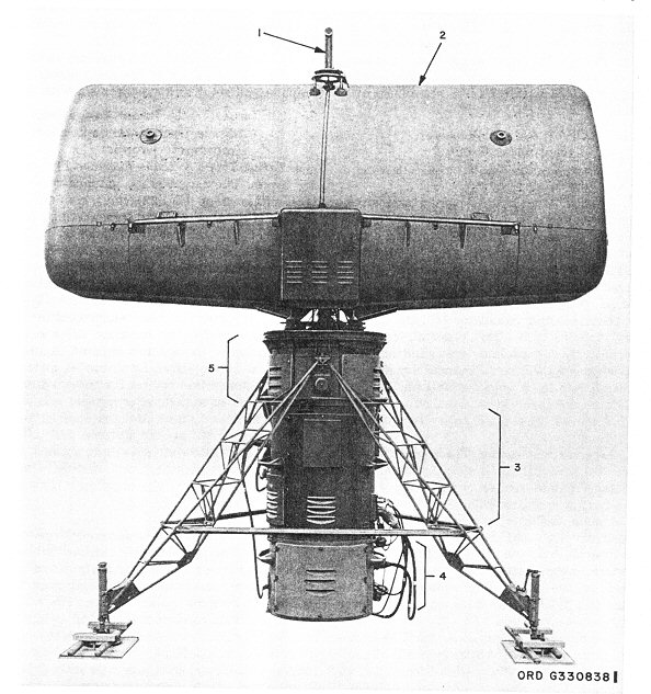
More details
- Auxiliary antenna [anti-jamming]
- Acquisition antenna
- Acquisition receiver-transmitter
- Acquisition modulator
- Acquisition antenna pedestal [drive motors, slip rings]
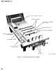
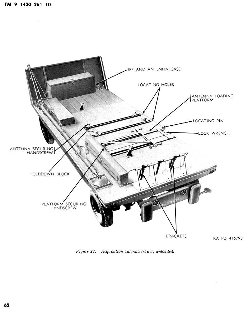
Operational equipment requires a surprising amount of support or transportation equipment. This just to carry that large odd shaped antenna safely. from Ezio Nurisio - website The LOPAR radar was very much like the original Nike Ajax (and M-33 gun) acquisition radar but with reduced pulses per second to match the longer range HIPAR radar or the ABAR radars mentioned above. It provided another "eye to the sky" and another problem for enemy jammers.
From Rolf Goerigk for the LOPAR include:
Polarization horizontal Antenna Gain CSC2 = 32 dB = 1600 ("CSC2" stands for co-secant squared, a vertical pattern optimized for aircraft detection at low and high altitudes and ranges) Beam Angle 1.4 deg Azimuth
2 to 22 deg. ElevationAntenna Speed 5, 10 and 15 RPM (Revolutions Per Minute) Azimuth Accuracy 1 deg. Noise 7.5 dB (1341 deg. Kelvin) Overall Noise 8 - 9 dB (1540-2014 deg. Kelvin) RF Freq. Range: 3.1 - 3.4 GHz RF Power average 650 W, peak 1 MW Pulse Width 1.3 microseconds Band Width IF = 4 MHz, Video=2 MHz Reflector Dimensions height 1.32 m, width 4.57 m, 5.6 sq. m To make life interesting, the Nike Ajax used a transmit pulse repetition Frequency (PRF)of 1000/sec, as per TM9-5000-9, and the Nike Hercules a PRF of 500/sec, as per MMS 150, 2-P5
For a more detailed description, see Lesson 2. LOPAR Acquisition Radar - 2.7 megabytes
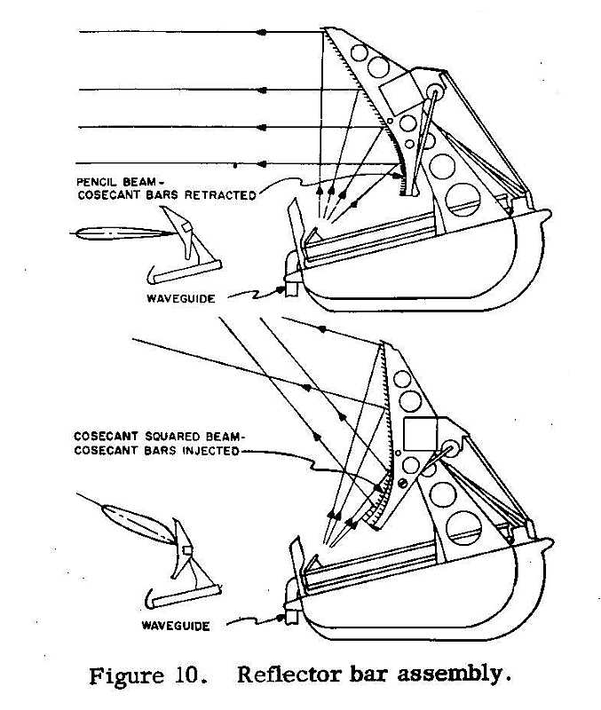
From Rolf Goerigk "As I first worked on site (1961). I was able to change the elevation by operating the ELEVATION switch on the ACQ control console and some hydraulic control under the ACQ-RADOM. During the early 60s the control was modified to electromechanical. It was possible to change elevation between 0 to 391 mils and to change the elevation mode too. Actually controlled was the point in mils when the cosecant-rods were driven in or out the lower part of the reflector, i.e. changing from pencil beam (long range) to cosecant (great height)."
LOPAR-Details from TM9-5000-9 Acquisition Radar Circuitry - 13.5 MByte - available this site.
Rotating Joint
This is how you connect a rotating rectangular wave guide in the rotating antenna with the fixed rectangular wave guide in the base ?? ;-))
This is a photo of a LOPAR slip ring assembly. The center copper tube is the outside of the rotating joint shown above. The multitude of metal rings are the slip rings. The glove finger tips gives a size comparison. 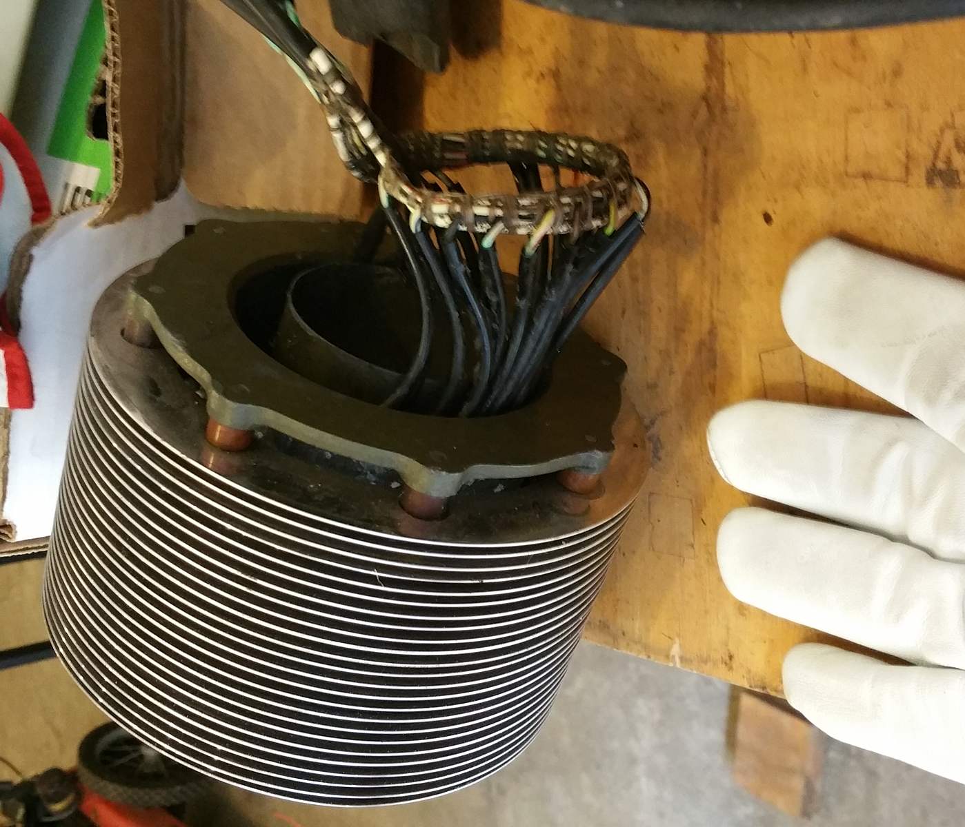
Another view of a LOPAR slip ring assembly. There are 24 slip rings (trust me ;-)
The LOPAR antenna looks and was rather unique :-)) Most 1940s-1970s antenna structures look rather parabolic. The parabolic surface in the LOPAR was hidden in the structure. The result was more compact, rectangular, and transportable. Nike was a "transportable" and "mobile" system :-)) With a battery of practiced men; maybe 6 hours disassembly and packup onto sufficient trucks, variable time for transportation, and 12 hours un-pack assemble setup and make functional. A few "mobile" Nike units practiced this, most Nike units were not considered "mobile" and never practiced moving their Nike site - a non-trivial exercize!!
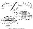
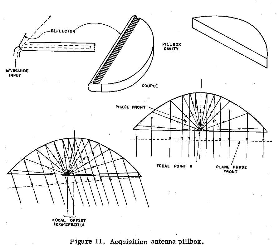
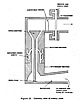
Parabolic Pill Box - In cross section below, converted the spherical radar waves from the feed-horn to flat radar waves for beaming into space. 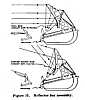
Reflector Bar Assembly - Formed the flat radar waves from above into a fan shaped beam, very narrow in azimuth (horizontal) say 1 degree). The LOPAR Acquisition Operator could adjust the elevation angle of the radar beam (about 20 degrees) and adjust its shape, less is needed high because aircraft are limited to about 100,000 feet. The cosecant bars adjusted the shape. 
The Acquisition Operator - could vary the vertical angles and patterns to maximize the radar return on targets of various altitudes by adjusting the LOPAR elevation angle and pattern.
Remember, for a given radar pulse peak power, (about one megawatt for the LOPAR) the radar return was proportional to 1/((target_range^4)*(target_crosssection^2))
(You can never get all the power you want ;-))
Acquisition Radar Displays, MTI, and Identification Friend or Foe (IFF)
The game plan is that the long persistence shows where the (airplane) was on previous sweeps.
Lets say the acquisition radar goes around once every 8 or 10 seconds -
you can see where the plane was for on towards the last 60 seconds.
(The tubes used the P7 phosphor.)
Even on displays 250 miles wide, there is a very visible comet trail where the plane has been.
This reveals to the eye the direction and relative speed.
The "ground clutter" shown on the above display can be a real problem in
some cases. The radar is sensitive to buildings, vehicles, mountains, trees, ...
for miles around. (For simplicity, the image above shows a trivial case.)
The Sensitivity Time Control (STC) reduced the gain of the receiver at close ranges so that
all return signals will have a more nearly equal intensity.
The Moving Target Indicator (MTI) system helped in suppressing the ground clutter
and enhancing moving objects (airplanes). This indeed worked/works
quite well in emphasizing airplanes and reducing the interference in viewing them
due to stationary objects. The system could be switched ON and OFF.
Several pages from TM9-5000-9 are on-line
(1.3 MByte) which further explains STC and MTI.
The "IFF" (Identification Friend or Foe)
Safe Lanes
Enemy or accidental jamming can/will cause many other interesting
displays on the tracking scopes. Go to jamming for
more information.
The tube that turned on the pulse of current to the magnetron in the
LOPAR Acquisition Radar Modulator (see above) took up to 15 minutes to warm up
to operate reliably and not risk damage. There was a 15 minute timer to
prevent operation (with a switch to override the timer in case of emergency).
The operator has a number of controls, the following are of special interest:
"Also in your information on IFF, the Aradcom had two types of IFF. The
standard IFF had a limited set of codes and you used a code of the day.
Generally all friendlies used the same code. In 1963 we also adopted
SIF/IFF which allowed enough codes for individual identification of aircraft
or flights of aircraft. The IFF sent a pulse out a few microseconds after
the radar. The aircraft responded with its pulse code. This difference in
delay is why a second bar was painted above the aircraft on the screen. The
IFF/and SIF had a particular code sequence for emergencies. When the pilot
switched to that code, it automatically painted four bars which was Mayday."
I know about SIF/IFF because during a simulation with the Air
Force in 1963, we accidentally engaged a flight of USAF planes. This caused
a stir when it was found that we had SIF installed but were still using the
old IFF. So I was sent with two other technicians from Fort Heath to a USAF
Radar Site in North Truro, Mass where USAF personnel trained us on the SIF
equipment.
Radar History
Wikipedia has a much more complete
History of radar
Return to beginning of Nike Radar
"Old style" band naming convention
Although the higher frequencies permit much smaller antennas to get the
same beam width, the higher frequencies suffer increasingly from
moisture in the air absorbing the radar waves. And also rain drops
reflect them more giving an effect similar to chaff. The choice of
radar frequency range for a particular application is a complicated compromise
involving many factors.
I remember in the 1950s folks were saying that radar was unaffected by weather -
I suspect the defense radar salesmen were touting that.
Our site on the lake front of Chicago was "socked-in" one foggy morning.
The whole lake that we could "see" with our acquition radar was solid white.
That never happened again in the two years I was there.
I don't know where I got this fragment:
Got that? Clear as mud? Need a memory aid?
Unlicensed radio frequency Industrial Scientific and Medical (ISM) bands
Regulatory authorities may allocate parts of the radio spectrum for unlicensed communications
that may or may not also be allocated as ISM bands.
RFID frequency bands - stolen from
Wikipedia Aug 26 2019
In case you are not confused enough already ?
Responding with "How far can you see?" - leads to a pointless discussion.
"But airplanes are in a more restricted size range."
True, 20 foot wing span to 200 foot wing span are most common. :-))
Let's "assume" the person asking the question is "thinking" of an aluminum
airliner or bomber, flying high enough so the curvature of the earth is not a problem.
Of course the real world is complicated :-((
There is a "defendable" answer, the "Presentation Range",
the maximum range of the radar presentation as seen by the radar operators.
Here is the detail for Nike Hercules TTR
You may notice that "stealthy" aircraft have lots of flat surfaces likely to reflect
a radar signal up, or down, but not back to the transmitting radar antenna.
If during an extreme manuver the aircraft accidently positions a flat surface towards the radar antenna,
it will be seen as an extremely large but very short time duration signal,
not likely to be seen again soon. This kind of signal return is difficult/impossible to track.
As a point of reference, the stealth fighter/bombers used in the Iraq conflict
are said by TV documentaries to have the radar reflectivity -"cross-section"- of a pigeon.
That seems an interesting accomplishment, as even one wheel of the aircraft
must have a much larger radar cross-section than a pigeon.
Accidental Jamming - Pulse Radars (used in Nike)
There are many friendly sources of radar interference.
Most folks worry about other friendly radars. However, these
are not a big problem at a typical Nike site, or even a
group of Nike sites very close together such as a Nike range at Red Canyon or McGreggor.
How can this be? Radars "shouting" all over the place,
and no problem? Unbelievable! But oddly enough, there is no big problem.
Here is why.
The attempt is not perfect, but usually about 95 % of the energy
gets directed as desired.
Nike radar magnetrons tune over a range of +- 5% from their center
frequency. And the receivers are tuned to be sensitive to roughly 0.1 % of that range.
In effect, about 500 radars in one band (+- 5% ) could be tracking one target
and not interfere with each other with respect to frequency.
Except - Nike site SF-59 was reported to be
jammed by the TV Channel 2 transmitter a half mile away.
Radar Jamming, Electronic Counter Measures (ECM)
The target may not wish to be observed, and/or may wish to reduce the
effectiveness of the radar attempting to observe it.
One way to reduce the effective range of the radar is to reduce the
reflectivity (ratio of energy reflected back) of the target.
This is called "stealth"
and is for aircraft designers, not us.
"Jamming" or "Electronic Counter Measures" (ECM) is a term used to describe
active means of trying to prevent the radar system from working as well as
intended. And of course radar designers actively try to defeat the ECM.
It is a great (but deadly) game of radar counter measures, counter-counter measures,
counter-counter-counter measures, played with very serious intent.
Documents, spotted by Greg Brown.
YouTube presentations - thanks to Greg Brown
Don Lee went to Electronic Warfare Countermeasures training in about 1968 (Added Dec 2020)
We will very briefly mention a few popular forms of
jamming:
There are whole groups of techniques for each of the above. And there are many
operational and equipment techniques used by the radar to try to counter the jamming
techniques. Jamming and counter jamming is an overwhelming complex field,
lets basically leave it alone in this introductory session. Just turning on your
radar transmitter and radiating can give the enemy interesting information for
present or future use. This game of cat and mouse is very interesting, and it is
not always certain who is the cat.
Modern Lessons :-))
Don Lee went to Electronic Warfare Countermeasures training in about 1968. (Added Dec 2020)
It got me off the mountain. I was the only US Army soldier in the class.
As you know In Pittsburgh The Air Force (USAF) would preform RBS runs "Radar Bomb Scoring" war games with us. RBS Games pitted USAF bombing and Army Air Defense crews practice and evaluate their technique and training. Cameras would record the jamming effectiveness on the radar display. used deception, repeater jammers to simulated new false aircrafts on the ground radar defense systems us. I do know, because of the commercial air traffic around Pittsburgh Airport the Air Force could not use its full jamming powers. Maybe that why they sent me so we could score better on the RBS games??
I was billeted in foreign pilot training dormitory. I was roomed with an Iranian cadet. Boy did the Air Force eat good, steak, etc. The Air Force had nice plates, tabled and settings. I remember getting back to my PI-43 barrack bunk and the not as good food and yes the extra duty. I was back in the real Army – vacation was over.
I left PI-43 as a SP4. Re-uping (short) for computer repair school at Ft. US Army Signal Corps School, Fort Monmouth NJ, for 11 months, then to Korea, Fort Benjamin Harrison IN, ending at, Headquarters Company, First US Army Defense Information School, Fort Meade MD.
You cover it very well at http://ed-thelen.org/ifc_acq.html#jamming. This training mostly improvement and sharpen my reaction times etc.
Good luck
From Peter De Marco
There are basically two types of radar jamming;
ECCM is an complex field and there are several operational and equipment techniques used by the ECCM Radar Operator to try to counter the jamming. The most important component of ECCM is the Radar Operator. The improper use of ECCM equipment and techniques can do more harm than good.
When the radar was being jammed there were several signal processing techniques that the ECCM Radar Operator could use to counter the jamming. Some of these methods are normally installed in radars to overcome natural phenomena such as weather or ground clutter, but they are all considered ECCM.
When the site was at Battle Stations or Blazing Skies it took two people to operate the ABAR equipment. One person was in the equipment room, which was located just below the radar dome. It was his job to keep the ABAR radar equipment peaked and running.
The other person operated the ECCM console, which was located in a room next to the Battery Control Van. It was his job to determine the type of ECM that was being used against the radar and to counter the effects of the jamming.
Since the range of the ABAR (about 200 nm) was greater than the LOPAR the ECCM Radar Operator would also call out targets that he was tracking to the Battery Control Van. The ABAR and the LOPAR were linked to the radar presentation in the Battery Control Van and the commander could switch from the LOPAR radar presentation to the ABAR radar presentation at his discretion.
The ECCM console could display six radar and two oscilloscope presentations at the same time. The main display showed what the ECCM Radar Operator considered the best radar presentation of the targets being tracked.
The other displays showed "previews" of the different types of ECCM presentations available. These ECCM presentations included "Dicke-Fix", "Side Lobe Blanking", "Slide Notch I-F Canceler", "Moving Target Indicator", etc.
By properly employing some or all of the above mentioned techniques the ECCM Radar Operator could significantly reduce the effects of ECM jamming.
For discussions of handling jamming in the Target Tracking Radars see:
Some of the nomenclature:
Impulsive noise, that can shock-excite the " narrow-band " radar receiver
and cause it to ring, can be reduced with the Lamb noise-silencing circuit,"
or Dicke fix." This consists of a wideband IF filter in cascade with a limiter,
followed by the normal IF matched filter. The wideband filter is designed
to include most of the spectrum of the interfering signal. Its purpose is to
preserve the short duration of the narrow impulsive spikes. These spikes
are then clipped by the limiter to remove a considerable portion of their energy.
If the large noise spikes are not limited and are allowed to pass they would
shock-excite the narrowband IF amplifier and produce an output pulse much
wider in duration than the input pulse. Therefore the interference would be in
the receiver for a much longer time and at a higher energy level than
when limited before narrowbanding. Desired signals which appear
simultaneously with the noise spike might not be detected, but the circuit
does not allow the noise to influence the receiver for a time longer than the
duration of a noise spike. This device depends on the use of a limiter. Limiters,
however, can generate undesired spurious responses and small-signal suppression,
and reduce the improvement factor that can be achieved in MTI
processors. It should therefore be used with caution as an ECCM device. 1f
incorporated in a radar, provision should be included for switching it
out of the receiver when it does more harm than good.
... Furthermore, at the higher frequencies the antenna sidelobe levels can be lower, making it
more difficult for sidelobe jamming. However, the advantages of operating against jammers at the higher
frequencies are balanced in part by the disadvantages of the higher frequencies, especially above L band,
for long-range air-surveillance radar.
The noise that enters the radar via the antenna sidelobes can be reduced by
coherent sidelobe cancelers. This consists of one or more omnidirectional antennas and cancellation circuitry
used in conjunction with the signal from the main radar antenna. Jamming noise in the omnidirectional
antennas is made to cancel the jamming noise entering the sidelobes of the main antenna." An antenna can also be
designed to have very low sidelobe levels to reduce the effect of sidelobe jamming. Low sidelobe antennas require
unobstructed siting if reflections from nearby objects are not to degrade the sidelobe levels.
By employing some or all of the above techniques, the effect of the sidelobe noisejammer can be significantly
reduced. Some of the above techniques can also reduce the jamming that enters via the main beam. The effects
of main-beam jamming can be further reduced by employing a narrow beamwidth to limit the region over which the
jamming appears. If the main beam cannot be made narrow because of constraints on the antenna size, an
auxiliary antenna can be employed to create a notch in the main-beam radiation pattern in the direction of the
jammer. With adaptive circuitry similar to that of the sidelobe canceler, this main-beam notch can be
automatically adjusted to be maintained in the direction of the jammer.
A web site involved with jamming is
EW Tutorial, Table of Contents
A book recommended by Aidan Fabius
via newsgroup sci.military.naval and Patrick Tufts
recommends
For further information, see "An Illustrated Guide To The
Techniques And Equipment Of Electronic Warfare"
There is a T1 manual on-line at
T1 AN/MPQ-T1
.pdf files - (7.5 Mbytes)
from Greg Brown, Oct 27, 2015
Electronic Warfare - DECEPTION JAMMING
INTRODUCTION
Deception jamming systems are designed to inject false information into victim radar to deny critical information on target azimuth, range, velocity, or a combination of these parameters. To be effective, a deception jammer receives the victim radar signal, modifies this signal, and retransmits this altered signal back to the victim radar. Because these systems retransmit, or repeat, a replica of the victim's radar signal, deception jammers are known as repeater jammers. The retransmitted signal must match all victim radar signal characteristics including frequency, pulse repetition frequency (PRF), pulse repetition interval (PRI), pulse width, and scan rate. However, the deception jammer does not have to replicate the power of the victim radar system.
A deception jammer requires significantly less power than a noise jamming system. The deception jammer gains this advantage by using a waveform that is identical to the waveform the radar's receiver is specifically designed to process.
Therefore, the deception jammer can match its operating cycle to the operating cycle of the victim radar instead of using the 100% duty cycle required of a noise jammer. To be effective, a deception jammer's power requirements are dictated by the average power of a radar rather than the peak power required for a noise jammer. In addition, since the jammer waveform looks identical to the radar's waveform, it is processed like a real return. The jamming signal is amplified by the victim radar receiver, which increases its effectiveness. The reduced power required for effective deception jamming is particularly significant when designing and building self-protection jamming systems for tactical aircraft that penetrate a dense threat environment. Deception jamming systems can be smaller, lighter, and can jam more than one threat simultaneously. These characteristics give deception jammers a great advantage over noise jamming systems.
Although deception jammers require less power, they are much more complex than noise jammers. Memory is the most critical element of any deception jammer. The memory element must store the signal characteristics of the victim radar and pass these parameters to the control circuitry for processing. This must be done almost instantaneously for every signal that will be jammed. Any delay in the memory loop diminishes the effectiveness of the deception technique. Using digital RF memory (DRFM) reduces the time delay and enhances deception jammer effectiveness. Deception jamming employed in a self-protection role is designed to counter lethal radar systems. To be effective, deception jamming systems must be programmed with detailed and exact signal parameters for each lethal threat.
The requirement for exact signal parameters increases the burden on electronic warfare support (ES) systems to provide and update threat information on operating frequency, PRF, PRI, power pulse width, scan rate, and other unique signal characteristics. Electronic intelligence (ELlNT) architecture is required to collect, update, and provide changes to deception jamming systems. In addition, intelligence and engineering information on exactly how a specific threat system acquires, tracks and engages a target is essential in identifying system weaknesses. Once a weakness has been identified, an effective deception jamming technique can be developed and programmed into a deception jammer. For example, if a particular radar system relies primarily on Doppler tracking, a Doppler deception technique will greatly reduce its effectiveness. Threat system exploitation is the best source of detailed information on threat system capabilities and vulnerabilities. Effective deception jamming requires much more intelligence support than does noise jamming.
Most self-protection jamming techniques employ some form of deception against a target tracking radar (TTR). The purpose of a TTR is to continuously update target range, azimuth, and velocity. Target parameters are fed to a fire control computer that computes a future impact point for a weapon based on these parameters and the characteristics of the weapon being employed. The fire control computer is constantly updating this predicted impact point based on changes in target parameters. Deception jamming is designed to take advantage of any weaknesses in either target tracking or impact point calculation to maximize the miss distance of the weapon or to prevent automatic tracking.
FALSE TARGET JAMMING
False target jamming is an effective jamming technique employed against acquisition, early warning, and ground control intercepts (GCI) radars. The purpose of this type of jamming is to confuse the enemy radar operator by generating many false target returns on the victim radar scope. When false target deception jamming is successfully employed, the radar operator cannot distinguish between false targets and real targets.
To generate false targets, the deception jammer must tune to the frequency, PRF, and scan rate of the victim radar. The jamming pulse must appear on the radar scope exactly like a radar return from an aircraft. Multiple false targets greater in range than the jammer are generated by delaying the transmission of a jamming pulse until after the victim radar pulse has been received. False targets closer in range are generated by anticipating the arrival of a radar pulse and transmitting a jamming pulse before the victim radar pulse hits the aircraft. If the victim radar employs a jittered PRF, only targets greater in range can be generated.
To generate different azimuth false targets, the deception jammer synchronizes its transmitted pulse with the victim radar's sidelobes. Due to their reduced power, when compared to the main beam, sidelobes are difficult to detect and analyze. The receiver in the deception jammer must be sensitive enough to detect these sidelobes and not be saturated by the power in the main radar beam. A false target deception jammer must inject a jamming pulse that looks like a target return into these sidelobes. To penetrate the radar sidelobes requires a lot of power. However, the power must be judiciously used. If a powerful jamming pulse is injected into the main beam, the false targets will be easy to detect. Most false target jammers vary the power in the jamming pulse inversely with the power in the received signal, on a pulse-by-pulse basis. This means the repeater jamming signal is at minimum power when the main beam of the victim radar is on the aircraft and at maximum power when the sidelobes are being jammed. To effectively generate false azimuth targets, the jammer must have a receiver with a wide dynamic range to detect both the main beam and the sidelobes. In addition, the jamming system must be able to generate high power that can be effectively controlled by the receiver.
To generate moving false targets, the deception jammer must synchronize with the main beam and the sidelobes in frequency, pulse width and PRF. Amplitude modulated jamming signals, with variable time delays, are transmitted into the sidelobes of the victim radar. The variable time delay provides a false target that changes range, either toward or away from the radar, depending on the time delay. The amplitude modulation provides false azimuth targets that appear to be moving.
The effectiveness of false target generation is based on the credibility of the generated false radar returns. If the victim radar can easily distinguish between false returns and target returns, the technique is a failure. The false returns must look identical to an aircraft return. The radar return on the victim radar scope should have the same intensity, depth, and width as a target return.
Power determines the false target intensity when it is displayed on the victim radar scope. Varying jammer output power inversely with received power ensures that each false target has nearly the same intensity as a true target return. The depth, or thickness, of the false target depends on the pulse width of the victim radar. By matching the pulse width of the jamming pulse with the pulse width of the victim radar, the jammer can generate false targets with the same depth as a real target return.
The width of the false target depends on the antenna pattern of the victim radar. This can pose a problem for false-target deception jammers. Because the jamming pulse is transmitted the entire time the radar beam is on the jammer, the width of a false target will tend to be greater than a real target return. Aircraft radar return varies with main beam cross-section. To correct this problem, most false target deception jammers use random modulation in the power of the transmitted pulses. This will vary the width of the false targets and make them look more like the variable returns of actual targets.
RANGE DECEPTION JAMMING
Although a specific TTR can track multiple targets and direct multiple weapons, the tracking circuit must select a single target return and track it while ignoring all other returns. Target selection is done by using gate bins. The range gate is used as the primary gate for target selection. A range gate is an electronic switch that is turned on for a period of microseconds based on a certain range or time delay after a pulse is transmitted
Range deception jamming exploits any inherent weakness in a TTR's automatic range gate tracking circuits. When a TTR's range gate locks on to an aircraft, the range deception jammer detects the radar signal. The range deception jammer then amplifies and retransmits a signal much stronger than the radar return. This retransmitted signal, called a cover pulse, is displayed in the range gate with the target signal.
The automatic gain control (AGC) circuit lowers the gain in the range tracking gate to control the amplitude of the cover pulse in the range gate. Reduced gain causes the real target return to be lost, and the range gate only tracks the jamming signal. This is known as range gate capture.
Once the range gate is captured by the cover pulse, a technique called range gate pull-off (RGPO) is employed. The deception jammer memorizes the radar signal and introduces a series of time delays before retransmitting. By increasing these time delays, the range gate will detect an increase in range and automatically move off to a false range. Once the range gate has moved well away from the real target, the range deception jammer shuts down, and the radar range gate is left with no target to track. The range gate breaks lock and the TTR must again go through the process of search, acquisition, and lock-on to re-engage the target.
There are several advantages of range deception jamming, especially when used as a self-protection technique. It can generate sufficient errors to deny range information and is effective against most automatic range tracking systems. This technique does not require a large amount of power, just enough to cover the radar return of the aircraft. If the time delays are not exaggerated, an operator may not detect the loss of range lock-on until after a missile has been fired. The insidious nature of range deception jamming may generate enough miss distance to save the aircraft and pilot.
There are disadvantages to using range deception jamming. First, it can be defeated by a trained radar operator. If the operator detects a problem with the automatic range tracking circuit, the system can be switched to manual range tracking mode to defeat RGPO. Also, if the threat system is still able to track the aircraft's azimuth and elevation, range information may not be required to complete target engagement. To maximize range deception jamming effectiveness, it should be employed in conjunction with azimuth and elevation jamming. Finally, this type of range deception jamming is not effective against a leading-edge range tracking system. A leading-edge tracker will not see the delayed cover pulse. As the cover pulse moves off the target, AGC circuits reset the gain to continue tracking the real target. The only way to defeat a leading edge range tracker is with a deceptive jammer that anticipates the next radar pulse and sends a jamming cover pulse before it reaches the aircraft. This jamming technique can also be defeated by randomly varying the radar PRF.
ANGLE DECEPTION JAMMING
Angle deception jamming is designed to exploit weaknesses in the angle tracking loop of the victim radar. The specific technique depends on the tracking method used to derive azimuth and elevation information. Inverse amplitude modulation jamming is the main angle deception technique used against TWS radars. For conical scan radars, scan rate modulation and inverse gain jamming are used. Swept square wave (SSW) jamming is used against LORO tracking radars.
The azimuth and elevation tracking loop for TWS radar is based on target signal amplitude modulation. The inverse amplitude modulation jammer generates a signal with modulation exactly opposite the expected return. To accomplish this, the angle deception jammer must receive the radar signals from the tracking beams. The jammer responds with a signal of the same frequency, PRF, and scan rate synchronized to the inverse of the radar antenna pattern. This induces an error in the angle tracking gate that, over a series of scans, causes the radar to lose target angle tracking.
Inverse gain jamming is also effective against conical scan radars. Since conical scan radars use the phase of the target returns to generate error signals, an inverse gain deception jammer attempts to alter the phase by inducing fake signals into the antennas. In addition, by altering the amplitude of the signal, the jammer induces large errors into the tracking loop. To accomplish this, the jammer must determine the frequency, PRF, and scan rate of the victim radar. It then transmits signals that change the phase and amplitude of the target signal, resulting in a signal 180 degrees out of phase with the actual target. This 180-degree error rapidly drives the antenna off the target and causes break-lock.
Scan rate modulation is also used against conical scan radars. This angle deception technique modulates the jamming pulse at or near the victim radar nutation frequency. As the modulation approaches the radar's nutation frequency, large error signals appear in the radar servo tracking loops, producing random gyrations in the antenna system, causing break-lock. This technique is most effective if the modulation jamming is slowly swept in frequency until it matches the nutation rate.
Both inverse scan and scan rate modulation jamming require very little power and have proven extremely effective against TWS and conical scan radars. To be effective, however, the angle deception jammer must find the precise scan rate of the victim radar. The jammer must concentrate on one signal at a time, limiting the number of threat systems that can be jammed simultaneously. In a dense threat environment, this can be a severe limitation.
The effectiveness of inverse gain and scan rate modulation jamming led radar designers to employ antennas that scan only during the receiving function of the radar system. Generally, this is accomplished by using two antennas. The transmitting antenna illuminates the target. Receiving antennas scan to produce the amplitude modulation of the reflected signal for effective angle tracking. This technique is called Lobe-On-Receive-Only (LORO). Since the transmitting antenna does not nutate, or scan, angle deception jammers cannot detect the modulation required to generate effective inverse gain modulation. Swept square wave (SSW) jamming is the angle deception technique developed to counter LORO angle tracking.
SSW jamming continuously varies the frequency of amplitude modulation on the jamming pulse over an expected range of nutation or scanning frequencies. This range is established by either electronic intelligence (ELINT) data on a particular system, or by exploitation. The dotted line in shows a threat's nutation or scan frequency. As the frequency of the modulated jamming pulse approaches the threat scan frequency, it induces errors in the angle tracking loop of the victim radar. The longer the SSW jamming stays near the scan frequency, the greater the induced errors. It is important that the sweep rate of the modulating jamming be slow enough to maximize its impact on the victim radar.
VELOCITY DECEPTION JAMMING
Pulse Doppler and continuous wave (CW) radars track targets based on velocity or Doppler-shifted frequency. The objective of velocity deception jamming is to deny velocity tracking information and generate false velocity targets. The primary techniques include velocity gate pull-off (VGPO), Doppler noise, narrow band Doppler noise, and Doppler false targets.
Velocity gate pull-off counters pulse Doppler or CW radars by stealing the velocity gate of their automatic tracking loop. The objective of VGPO is to capture the Doppler velocity tracking gate by transmitting an intense false Doppler signal. Then the frequency of the false signal is changed to move the tracking gate away from the true target Doppler. This is analogous to the RGPO technique used against the range gate tracking loop.
To accomplish an effective VGPO technique, the jammer receives the CW or pulse Doppler signal. It then retransmits a CW or pulse Doppler signal that is higher in power than the return from the aircraft, but at approximately the same Doppler frequency. It is important that the frequency of this initial jamming pulse appears within the same velocity tracking filters as the target return or the victim radar will disregard it. The frequency band of the Doppler tracking filters is an important piece of intelligence information. The velocity tracking gates are quite narrow, roughly 50 to 250 MHz. Once the jamming pulse appears in the tracking gate, the automatic gain control circuit gains out the target return, and the jamming pulse has captured the velocity gate.
Once the jamming pulse has captured the tracking gate, the deception jammer slowly changes the Doppler frequency. This frequency shift is accomplished by several methods. The most common method uses frequency modulation (FM) within the jammerís traveling wave tube (TWT). By varying the TWT voltage, the Doppler frequency of the jamming pulse is changed linearly, and the radar tracking gates follow the jamming pulse. By using FM, the jamming pulse can be moved in either a positive or negative direction, depending on the slope of the voltage. By slowly changing the frequency of the modulation, the jamming pulse pulls the tracking gates off the target. When the maximum offset has been achieved, nominally 5 to 50 kHz, the FM is ìsnapped backî to a minimum value, and the process is repeated to preclude target reacquisition.
The rate of change of frequency offset in a VGPO pulse is an extremely critical parameter. Many CW and pulse Doppler radars employ acceleration stops as part of the tracking gates. By differentiating the velocity outputs of the velocity tracking gates with respect to time, the velocity tracker computes target acceleration. Acceleration stops detect and reject unusually large changes in target acceleration. If the VGPO technique changes the frequency of the jamming pulse too rapidly, the tracking loop, with acceleration stops, will reject the jamming pulse and stay on the target. This means that an effective VGPO technique may take from one to ten seconds.
Doppler noise differs from most noise techniques in that it is a repeater technique. The jamming system must receive the pulse Doppler radar signal in order to generate an appropriate jamming pulse. Also, noise jamming output is done on a pulse-by-pulse basis and only lasts as long as the pulse duration, or pulse width, of the victim radar signal. The Doppler noise jammer receives each pulse and applies a random frequency shift, either positive or negative, to each pulse.
When Doppler noise jamming pulses are processed by the signal processor, and the Doppler frequencies are sent to the velocity tracking gate, there are so many different velocities that the tracking gate cannot distinguish the target from the jamming. The random distribution of target velocities effectively masks the true target Doppler velocity. If the velocity tracking loop is not saturated, multiple false targets traveling at different speeds will be displayed.
When a technique called Doppler noise blinking is employed, it interferes with the angle and velocity tracking within most semi-active radar missiles. Doppler noise blinking is accomplished by rapidly transmitting bursts of Doppler noise jamming.
Doppler noise jamming is effective against most pulse Doppler radars and the semi-active missiles employed with these radars. One disadvantage, however, is that it is only effective against the velocity tracking loop. If range tracking is still available to the radar, Doppler noise may highlight the jamming aircraft. Another disadvantage is that Doppler noise requires a sophisticated jammer able to receive the victim radar pulse, generate random positive and negative frequency modulations on this pulse, and retransmit the jamming pulses at the PRF and pulse width of the victim radar. This requires an extremely fast signal processing capability and detailed intelligence information on the victim radar.
Narrowband Doppler noise is also a repeater technique. The jamming system receives the pulse Doppler radar signal and generates a noise jamming signal on a pulse-by-pulse basis . Narrowband Doppler noise requires detailed information on the frequency coverage of an individual velocity tracking filter, or velocity bin, employed by the victim radar. Once this frequency range is known, the jammer receives each pulse from the victim radar and transmits jamming pulses with a higher and lower frequency shift based on the real target Doppler. These frequency shifts are always within the frequency range of the velocity bin.
When these pulses are processed by the signal processor and the Doppler signals are sent to the velocity tracking gates, the particular bin that contains the target Doppler also contains several other targets generated by the jammer. The victim radar signal processor attempts to distinguish the target Doppler from the jamming pulses. It raises the gain in the velocity tracking bins, thinking that the signal with the highest amplitude is the target. But, as the signal gain is increased, the target is ìgained outî with the jamming signals and no target is displayed. This is called velocity bin masking and can completely deny target information to a pulse Doppler radar.
The advantage of narrowband Doppler noise is that it completely masks an aircraft's velocity from a pulse Doppler radar. The disadvantages include the following: When the victim radar can range-track an aircraft, narrowband Doppler noise highlights the aircraft's presence. To be effective, narrowband Doppler noise requires knowledge of the frequency range of the victim radar's velocity tracking bins, or filters. This detailed information may be available only through threat system exploitation. Finally, sophisticated signal processing and jamming systems are required to receive and transmit in the very narrow frequency band of the velocity bin.
Doppler false target jamming is normally used with narrowband Doppler noise or other deception techniques. Its purpose is to initially confuse the radar signal processor with multiple targets and then force the radar signal processor to raise its gain levels in the velocity tracking loop. The Doppler false target jammer receives each pulse of the victim radar and applies a random frequency shift to a selected number of these pulses.
The selected pulses are processed by the signal processor, and multiple Doppler frequencies are sent to the velocity tracking gate. In an attempt to distinguish the target from the jamming pulses, the signal processor increases the gain in each tracking filter, assuming the target Doppler has a higher amplitude than the jamming pulses. This increase in gain sets up the velocity tracking loop for a narrowband Doppler noise technique that will cause the real target to be lost among the generated false targets.
The advantage of Doppler false target jamming is that it can initially confuse the radar signal processor and the radar operator as to the velocity of the real target. It also sets up the radar for narrowband Doppler noise technique and increases its effectiveness. The disadvantage is that the signal processor or the radar operator will eventually be able to distinguish the real target from the false targets based on its velocity. This jamming technique is much more effective when used in conjunction with other Doppler jamming techniques.
MONOPULSE DECEPTION JAMMING
The ability of monopulse tracking radars to obtain azimuth, range, and elevation information on a pulse-by-pulse basis make them extremely difficult to jam. Amplitude modulation jamming used against conical scan or TWS radars, such as inverse scan and swept square wave, highlights a target, making monopulse tracking easier. Frequency modulation techniques, such as RGPO and VGPO, are equally ineffective. They serve as a beacon that aids the monopulse radar's target tracking ability. The monopulse radar may be able to track the jammer with more accuracy than tracking actual radar returns because target glint effects are absent from the jamming pulse. Monopulse angle jamming techniques can be divided into two main categories, system-specific and universal. Examples of system-specific jamming techniques include skirt frequency jamming, image jamming, and cross-polarization jamming. These techniques attempt to exploit weaknesses in the design and operation of specific monopulse radars. Cross-eye jamming, a universal technique, attempts to exploit all monopulse radar systems.
Skirt frequency jamming, or filter skirt jamming, is designed to counter the monopulse receiver. Skirt frequency jamming is based on the fact that the intermediate frequency (IF) filter of the monopulse receiver must be correctly tuned to the transmitting frequency of the monopulse radar. It these two components are not exactly tuned, the target signal may be presented on the edge, or skirt, of the receiver IF filter. This offers an opportunity to inject a jamming signal into this skirt
Filter skirt jamming attempts to take advantage of this frequency imbalance by transmitting a jamming pulse tuned slightly off the radar transmitted frequency and in the middle of the receiver IF filter. This jamming pulse will generate a false error signal and drive the antenna away from the true target return.
A well designed and maintained monopulse system does not have a frequency imbalance. The transmitter and IF filter frequencies will be identical. Jamming signals that are even slightly out of this narrow frequency range will not affect the monopulse tracking capability of the radar.
Effective filter skirt jamming requires extensive knowledge of the internal operation of the IF filter. This information can normally be obtained only by system exploitation. Variances from radar to radar and frequency imbalance exists from one radar IF filter to another. This creates a high degree of uncertainty in the effectiveness of this technique.
Image jamming exploits another potential weakness in the monopulse receiver. Some monopulse receivers have a wide-open front end with no preselection before the mixer. If the jammer transmits a pulse at the intermediate, or image, frequency, but out of phase with this frequency, the phase of the target tracking signal will be reversed and the antenna will be driven away from the target. Effective image jamming requires detailed information on the operation of the monopulse receiver. Of particular importance is the image, or intermediate, frequency and whether the local oscillation frequency is above or below the transmitted frequency. This may require exploitation of the monopulse threat system. In addition, a well-designed monopulse system has preselection in the front end and will reject signals that are out of phase with the transmitted frequencies. This capability renders image jamming ineffective.
Cross-polarization jamming exploits the difference in the monopulse antenna pattern for a jamming pulse that is polarized orthogonal to the design polarization. The antenna pattern for a two-channel monopulse radar using sigma and delta beams shows the tracking point to be between the two beams .This is true if the radar is using its design polarization. However, the radar antenna also has a receiving pattern for a signal that is cross-polarized with the design frequency. For a cross-polarized signal, the tracking point is shifted one beamwidth to the right. This shift in the tracking point results in a target tracking signal that is 180∞ out of phase with the real signal. To be effective, a jamming signal polarized orthogonally to the design frequency of the radar would have to be 25 to 30 decibels, or about 1000 times, stronger than the radar signal.
A cross-polarized jammer must receive and measure the polarization of the victim monopulse radar. The jammer then transmits a very high power jamming signal at the same frequency, but orthogonally polarized, to the victim radar. As a rule, the jamming signal must be 25 to 30 dBs stronger than the target return to exploit the tracking errors in the cross-polarized antenna pattern. Additionally, it must be as purely orthogonal to the design polarization as possible. Any jamming signal component that is not purely orthogonal will highlight the target and require more jamming power to cover the target return.
A cross-polarized jammer must be able to generate a powerful jamming pulse that is polarized orthogonal to the victim radar. A cross-polarized jammer that generates the power and purity of polarization required to defeat monopulse angle tracking poses extreme technological challenges.
Cross-eye jamming is a complex technique that attempts to distort the wavefront of the beams in a monopulse radar and induce angle tracking errors. It exploits two basic assumptions of monopulse tracking logic in comparing target returns on a pulse-by-pulse basis. The first assumption is that a target return will always be a normal radar pulse echo. The second assumption is that any shift in amplitude or phase in a target return is due to the tracking antenna not pointing directly at a target. This condition generates an error signal and the antenna tries to null, but the amplitude or phase shifts.
Cross-eye jamming attacks the two assumptions through a process of receiving and transmitting jamming pulses from different antennas separated as far apart as possible.The phase front of a monopulse signal is received by the number 1 receive antenna, amplified by the repeater, and transmitted by the number 2 transmit antenna. The same phase front then hits receive antenna number 2, is shifted 180∞, amplified by the repeater, and transmitted by the number 1 transmit antenna. These two out-of-phase signals must be matched in amplitude and must exceed the amplitude of the target return.
When these jamming signals arrive at the victim radar, the tracking loop attempts to null out the amplitude and phase differences. With two widely spaced jamming sources at different phases, the antenna never achieves a null position or tracking solution. The distance between antenna pairs is an important parameter that determines the effectiveness of cross-eye jamming. The wider the spacing between antenna pairs, the more distortion in the victim's wave front near the true radar return. Most fighter aircraft do not provide sufficient spacing between the antennas to maximize effectiveness. Effectiveness is also lost when the aircraft is abeam or going away from the radar. To further complicate matters, when the radar is directly in front of the aircraft, the jamming pulses must have a power at least 20 dBs above the target return. Cross-eye jamming can also be defeated with a leading-edge tracker that rejects jamming signals arriving at the antenna behind the target return.
Countering monopulse angle tracking is the greatest challenge for selfprotection jamming systems. Skirt jamming and image jamming have had limited success. Cross-polarization and cross-eye jamming techniques require complex and sophisticated circuitry and much power.
TERRAIN BOUNCE
Terrain bounce is a jamming technique used primarily at low altitude. It is used to counter semi-active, air-to-air missiles and monopulse tracking radars. The technique involves a repeater jammer that receives the radar or missile guidance signal. The jammer amplifies and directs this signal to illuminate the terrain directly in front of the aircraft. The missile or radar tracks the reflected energy from the spot on the ground instead of the aircraft.
To be effective, the terrain bounce jamming antennas should have a narrow elevation beamwidth and a broad azimuth beamwidth. This transmission pattern maximizes the energy directed toward the ground and minimizes the energy transmitted toward the missile or radar. To overcome signal losses associated with uncertain terrain propagation, the jamming system should also generate high jamming power. This ensures the energy reflected from the terrain is higher than the energy in the aircraft return. The terrain bounce jamming antennas should have very low sidelobes to preclude activation of any home-on-jam (HOJ) missile capability. For an air-to-air missile, the terrain bounce technique should be activated at long range. This will initially put the aircraft and the jamming spot in the same resolution cell. As the range decreases, the missile will be decoyed by the higher power in the jamming spot.
Some problems associated with terrain bounce jamming include the uncertainty of the signal scattering parameters of the various terrain features and the possible changes in signal polarization caused by terrain propagation. In addition, terrain bounce jamming can place maneuvering restrictions and maximum altitude limitations on the aircraft.
SUMMARY
There is several deception jamming techniques that can be employed to counter threat radar systems. The effectiveness of these techniques can be enhanced when they are employed in combination. For example, the effectiveness of an RGPO technique is enhanced when an angle deception technique is also employed. Determining the most effective deception technique, or combination of techniques, can present a challenge to intelligence and engineering analysts. However, when employed with maneuvers and chaff, deception techniques can mean the difference between success and failure on the modern battlefield.
In principle the aircraft being illuminated by the radar permits one of the
aircraft's ARM missiles to lock onto that radar, and the aircraft can then
"launch and forget" the ARM missile. The illuminating radar may be able to
see the very small "radar cross section" of the missile at closer ranges,
especially if the missile is currently in the major lobe of the radar.
I understand that that ARMs were used successfully in the Gulf War, if not previously.
Unfortunately, at the present time I know nothing about them.
And then Bill Cahill
responded to the above:
The Shrike, built by Texas Instruments, had different variants
designed to home in on different frequencies. If the radar went off the
air, the missile went stupid. The Shrike was essentially an air launched
version of a semi-active radar homing surface to air missile, homing in on
the target radar instead of a target illuminated by a host radar. Shrikes
were effectively used by the US in Vietnam and Israel in the Middle East.
The AGM-78 Standard ARM augmented the Shrike in 1968, providing greater
range and mission flexibility. The Standard was improved over the next 10
years, with many variants entering service with the USAF and USN. Unlike
the Shrike, the Standards can 'remember' where a radar is even if it ceases
transmission. The ultimate (to date) ARM, the HARM, entered service in the
mid 1980s. This high speed, maneuverable missile is currently in inventory
with the USAF and USN and has replaced the Shrike and Standard.
And then Nicholas Maude
responded to the above:
U.S. Artillery also uses measurements of historical significance. These units were
in use 40 years ago.
In 1997, I asked Col. Moeller - MoellerS@ssdch-usassdc.army.mil -
if these units were still in use. He kindly responded as follows:
and "We us standard US weather lingo, definitely F, not C."
The information from surveillance radar is customarily displayed
with the "Plan Position Indicator"
tube, abbreviated to "PPI scope". This is the big round CRT (TV) tube with the
sweep going around all the time. Basically, you and the radar set are in the middle of this
big round map, and the radar us showing you what is going on around you.
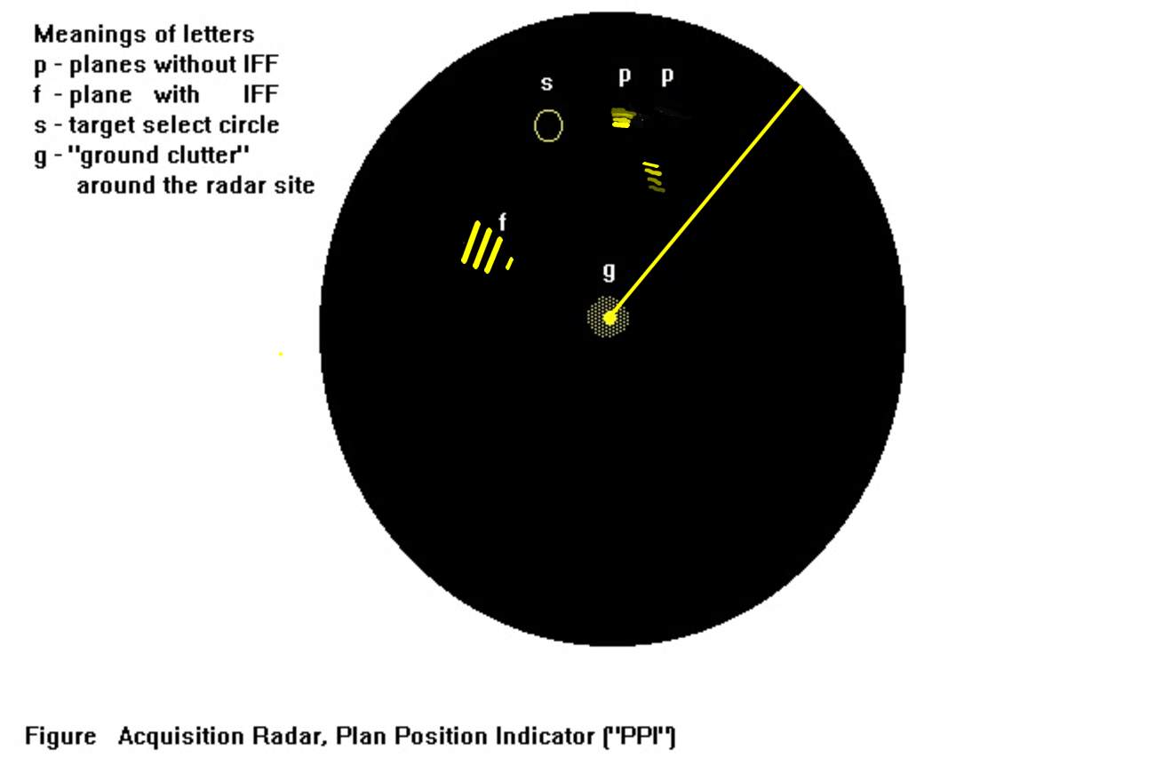
(On the above diagram, only the planes are shown with the delayed phospher effect.)
A related AN/TPS-1G Moving Target Indicator manual.
is basically a series of coded pulses sent
out at the same time and same direction as the surveillance radar pulse.
It was sent out by separate IFF equipment. A "friendly" unit was equipped to respond to
the coded pulses with another set of coded pulses. These were received by the
IFF equipment, and usually displayed with the surveillance radar display.
The system resembles the methods FAA aircraft controllers use to track commercial
and other suitably equipped aircraft, EXCEPT that the military codes
are secret and change often (possibly daily).
And what about friendly aircraft without functioning IFF equipment. Say equipment malfunction,
including having Foe bullets through your IFF transponder (receiver and transmitter)??
There must be contingency plans/methods to cover these situations. One of the methods is
to have "safe lanes" for friendly aircraft (with possibly malfunctioning IFF equipment)
to get from say the combat area back to a friendly airfield. Often these are marked in
"grease pencil" on charts and/or PPI scopes. These safe lanes are of course secret, or should be.
 IFF Symbols and FUIF sysbols with text.
50,000 yards (about 28 miles)
150,000 yards (about 85 miles)
250,000 yards (about 140 miles)
350,000 yards (about 200 miles)
Although some very long range radars (such as Nike HIPAR) were fixed at about 7 RPM
From Robert Noakes March, 2001
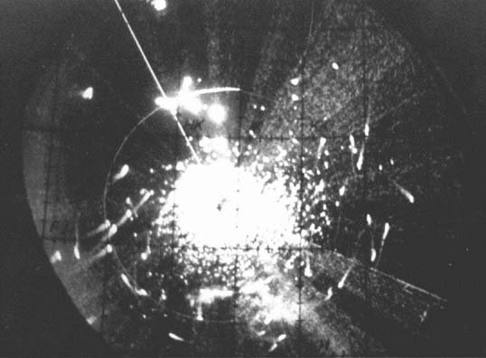
A PPI display with planes and jamming image is 35 K bytes.
(Photo credit Rolf Goerigk
There are various unverified stories that in practice combat between the
Air Force with their jamming equipment, and the Nike with their anti-jamming
equipment, that the Nike successfully tracked the Air Force planes and would
have had successful intercepts with the Hercules missiles.
This was reputed to be true even when the Air Force used their best jamming equipment
to try to confuse the tracking.
Pictures of MTI chassis and delay line
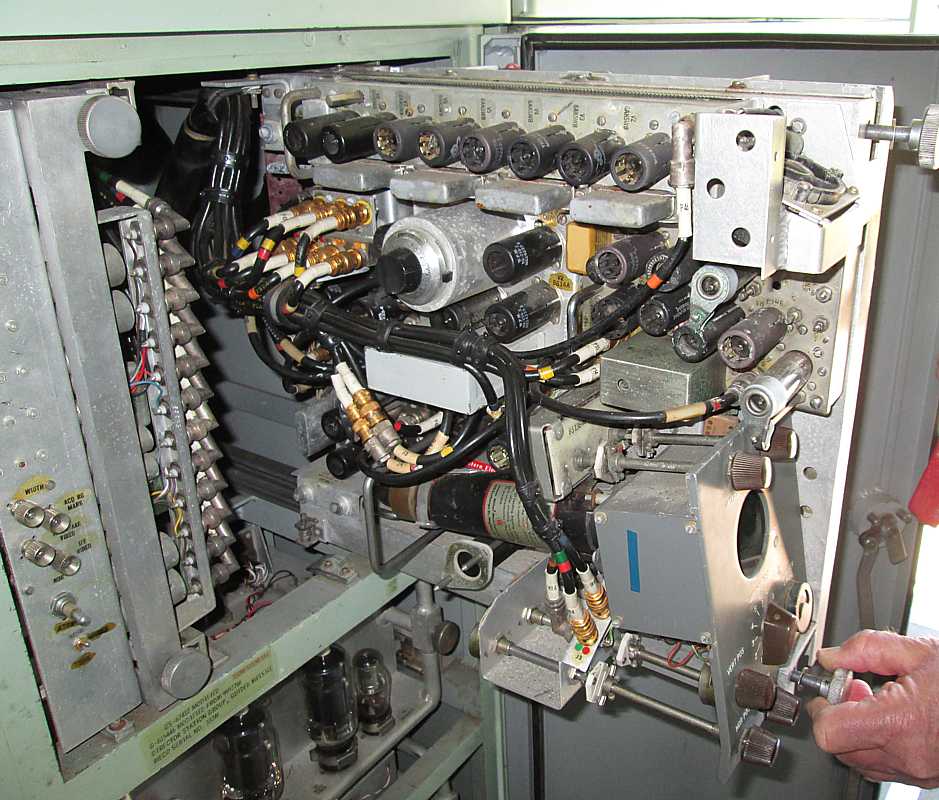
This is the Moving Target Indicator chassis in the BC van at SF-88 for the Hercules system.
The Ajax MTI did not have so many adjustments nor dedicated scope.
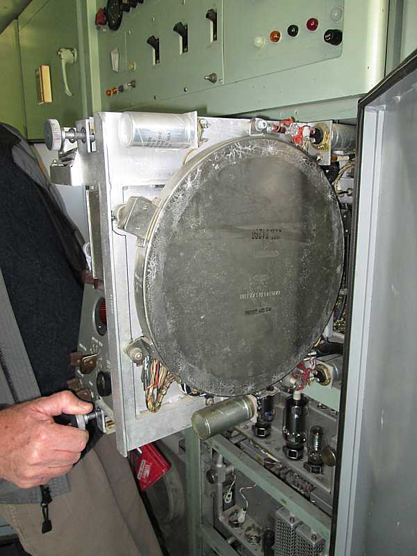
The MTI delay line on back side of the MTI chassis. The Ajax delay line
was a seventeen sided quartz crystal with a delay time of 1 millisecond.
The acquisition pulse repetition frequency was synchronized with this delay line.
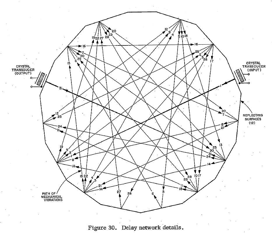
This is a schematic of a 15 sided delay line from another radar.
The following is from "Radar Technology", edi. Eli Brookner,
(C) 1977 ARTECH HOUSE, INC. ISBN 0-89006-021-5
1886-1888 Heinrich Hertz demonstrates generation, reception,
and scattering of electromagnetic waves
1903-1904 Christian Hulmeyer develops and patents a primitive
form of collision avoidance radar for ships
1922 M.G. Marconi (in acceptance speech for an honor)
an angle-only radar for ship collision avoidance
1925 First short pulse echoes from the ionosphere are
observed on CRT by G. Breit and M. Tuve of
Johns Hopkins University
1934 First photo of short pulse echo from aircraft made
by R.M. Page of Navel Research Lab.
1935 First demonstration of short pulse range
measurements of aircraft targets, by British and Germans
1937 First operational radar built - the Chain Home in
Britain, designed by Sir Robert Watson-Watt
1938 Signal Corps SCR-268 becomes first operational
anti-aircraft fire control radar; 3100 sets eventually produced,
Range, > 100 mi.; freq, 200 MHz
1938 First operational shipboard radar, the XAF, aboard the
battleship USS New York, 12 mi ships, 85 mi aircraft
1941-Dec By this date, 100 SCR-270/271 Signal Corps early
warning radars have been produced. One of these radars,
located (near) Honolulu, detects Japanese planes approaching Pearl Harbor ...
Radar Frequency Bands

Worldwide Spectrum Allocations from Tektronix - (1.2 MByte) - via Kevin Appert - 2022
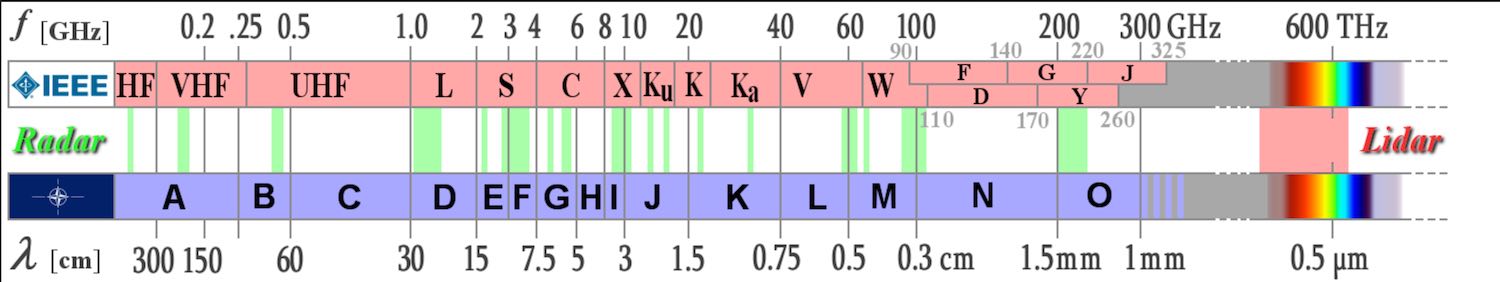
https://www.radartutorial.eu/07.waves/Waves%20and%20Frequency%20Ranges.en.html - 2021
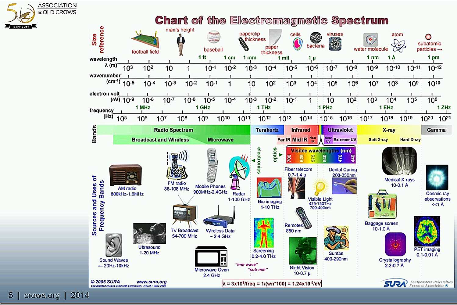
Electromagnetic Frequency Spectrum, from "Old Crows"
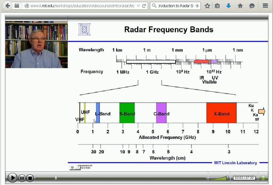
Radar Frequency Bands
from http://www.ll.mit.edu/workshops/education/videocourses/introradar/lecture1/part2/
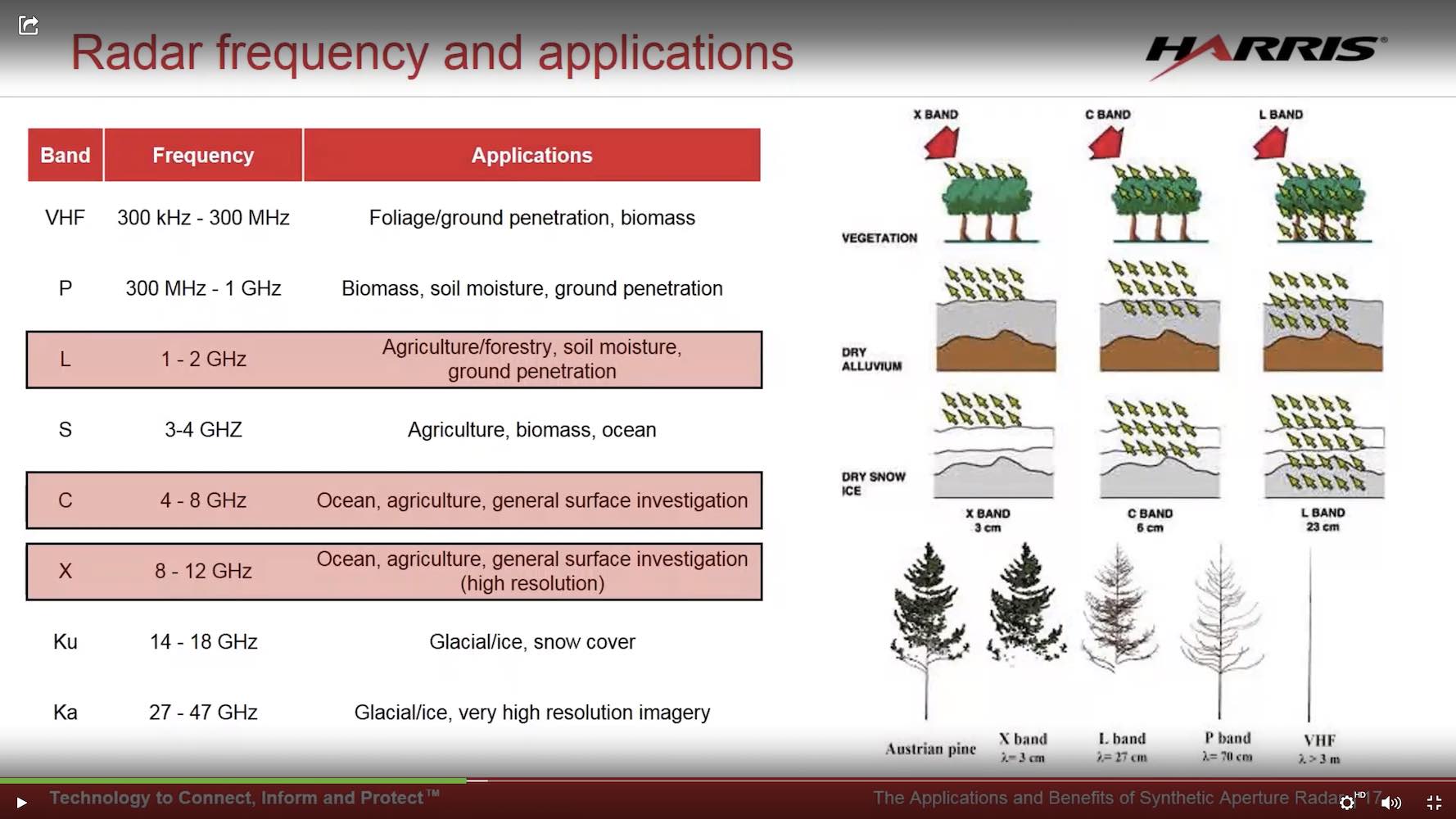
Synthetic Aperture Radar - Frequency Use
from L3Harris Geospatial, webinar

Atmospheric Opacity, from a SETI presentation -
The Breakthrough Initiative - Listen and Megastructures at KIC 8463 - Andrew Siemion (SETI Talks)
https://www.youtube.com/watch?v=jDT6E4SbVow

The Apollo Unified S Band Communications System
Excellent article about frequencies and techniques
used in the Apollo moon landing systems - via Carl Claunch
local copy

Cell Phone Frequencies by Nation
from https://www.gresham.ac.uk/lectures-and-events/cell-phones
Wavelength in cm ~ 30,000 / frequency in MHz
Band
Frequency(MHz)
Wave Length
Comments & common usage
-
20-55
about 10 meter
British Chain Home (helped win Battle of Britain, 1940) had anti-jamming
tools - also https://www.youtube.com/watch?v=FQserKrZXqU
-
500
60 cm
Germany Freya - 1940
VHF
214- 236
130 cm
?
P
300
100 cm
?
UHF
425- 610
60 cm
BMEWS (ballistic early warn), PAVE PAWS
L
1250-1380
23 cm
Airport Surveillance, Nike HIPAR acquisition
- L5
- L2
- L1
1176.45
1227.6
1575.42
about 20 cm
GPS - IIA - - (Much GPS information on the Internet !! )
GPS - P(Y) - military & dual-freq. (models ionosphere delays)
GPS - C/A, P(Y) - civilian single channel - gps.gov
.
1,421
21.11 cm
Hydrogen Hyperfine Split (Radio Astronomy)
and watched by SETI@home.
1420 MHz to 1666 MHz
"water hole",
especially interesting to
radio astronomers and SETI folks
S
2217.5 MHz
2380
2,400-2,500
2,450
2,491.75
12 cm
ICE spacecraft,
International Cometary Explorer
Arecibo - asteroid radar - 900 KW - duty cycle approaches 50%
one of the
ISM (industrial, scientific and medical) bands
802.11G WiFi, Bluetooth, cordless phones, ...
Zigbee is used by Calif. PG&E to turn off your AC to help keep the lights working on peak loads.
"Zigbee operates in the industrial, scientific and medical (ISM) radio bands: 2.4 GHz in most jurisdictions worldwide; ..."
(magnetron in your microwave oven)
Chinese BeiDou-1 navigational satellites in geostationary orbit.
S
2700-3900
10 cm
Sage, DEW line, Nike LOPAR acquisition (3.1-3.4 Ghz)
C
5300-5520
5 cm
Height Finder, Patriot
8560
3.5 cm
Goldstone - asteroid radar - 450 KW - duty cycle approaches 50%
X
9230-9404
3 cm
Precision Approach, Nike Target Tracking (TTR)
Ku
12,000-18,000
18 mm
Nike Target Ranging Radar (TRR), Mortar-location, StarLink ?, circular polarization
K
20,000
15 mm
?
.
22,000
13.6 mm
minor H2O absorption line
.
24,000-24,250
12.5 mm
automotive radar - (SSR-Short Range Radar, blind spot detection,
lane change and backup, stop-and-go and parking warning)
.
31,500
10.5 mm
(Cosmic Background - "Big Bang")
Ka
27,000-40,000,000
8.5 mm
nominal upper limit of traditional radar, StarLink ?, circular polarization
.
37,000-43,500
8 mm
5G communication
Q
"millimeter"
40,000
7 mm
used in outer space
.
60,000
5 mm
major O2 absorption line, fog (clouds) becomes a major problem
V
40,000-75,000
StarLink ?, circular polarization
E
(?modern
name)
77/79 GHz
4 mm
automotive radar - (LRR- Long Range Radar, cruise control & emergency brake) & local data transfer
an interesting article
.
227.1 and
229.1 GHz
1.3 mm
The Event Horizon Telescope Collaboration, global very long baseline interferometric observations
image "black hole", 2017 observing run
First M87 Event Horizon Telescope Results. III. Data Processing and Calibration
The Astrophysical Journal Letters, Volume 875, Number 1
Radio Frequency Naming Convention
Band
Frequency(MHz)
A 0 - 250
B 250 - 500
C 500 - 1000
D 1000 - 2000
E 2000 - 3000
F 3000 - 4000
G 4000 - 6000
H 6000 - 8000
I 8000 - 10000
J 10000 - 20000
K 20000 - 40000
L 40000 - 60000
M 60000 - 100000
Radio Frequency Naming Convention
Band
Designation
EVLA
Frequency
Range (GHz)
4 73.5-74.5 MHz
P 300-340 MHz
L 1.0-2.0
S 2.0-4.0
C 4.0-8.0
X 8.0-12.0
Ku 12.0-18.0
K 18.0-26.5
Ka 26.5-40.0
Q 40.0-50.0
The 10 Frequency Bands of the ALMA antennas
at
Atacama Large Millimeter/submillimeter Array
ALMA Band
Frequency
Range
(GHz)
Receiver Noise
(K) over 80%
of the RF band
1 31 - 45 17
2 67 - 90 20
3 84 - 116 37
4 125 - 163 51
5 162 - 211 65
6 211 - 275 83
7 275 - 373 147
8 385 - 500 196
9 602 - 720 175
10 787 - 950 239
Global Navigation Space Systems - center frequencies
GPS
MHz
L1 1575.42
L2 1227.6
L5 1176.45
GLONASS
MHz
M 1602.00
+.n◊0.5625 MHz
K1 1246.00
+ n◊0.4375 MHz
L1OC 1600.995
L2OC 1248.06
L3OC 1202.025
L1OCM 1575.42
L3OCM 1207.14
L5OCM 1176.45
Galileo
MHz
E1 1575.42
E5A 1176.45
E5 1191.795
E5D 1207.14
E6 1278.75
BeiDou-1
MHz
B1 1561.1
B2 1207.14
B3 1268.52
Weather Radar Frequencies
as per Wikipedia
These modern systems
Ground based 10 cm to 5 cm
Aircraft based 3 cm
are very sophisticated
- microprocessors
- large memories
- sophisticated algorithms
Wikipedia seems to do a good job on
weather radar.
"The DPR consists of Ku-band (13.6GHz) and Ka-band
(35.5GHz) channels. A major source of error in the rainfall estimates from the TRMM/PR comes
from the uncertainty in the conversion of radar re
ectivity into rainfall rate. This uncertainty
originates in the variations of the raindrop size distribution (DSD) that changes by region, season
and rain type. One of the reasons for adding the Ka-band frequency channel to the DPR is to
provide information on the DSD that can be obtained from non-Rayleigh scattering effects at
the higher frequency.
Another reason for the new Ka-band"
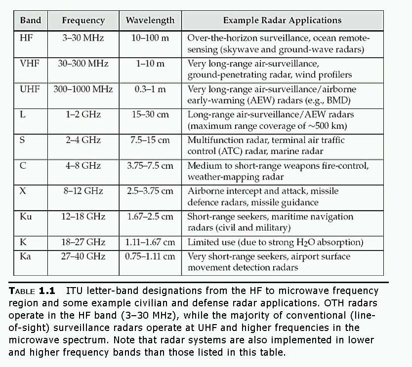
from wikipedia
Frequency range
Bandwidth
Center frequency
Availability
6.765 MHz
6.795 MHz
30 kHz
6.780 MHz
Subject to local acceptance
13.553 MHz
13.567 MHz
14 kHz
13.560 MHz
Worldwide
26.957 MHz
27.283 MHz
326 kHz
27.120 MHz
Worldwide
40.660 MHz
40.700 MHz
40 kHz
40.680 MHz
Worldwide
433.050 MHz
434.790 MHz
1.74 MHz
433.920 MHz
Region 1 only and subject to local acceptance
(within the amateur radio
70 cm band)
902.000 MHz
928.000 MHz
26 MHz
915.000 MHz
Region 2 only (with some exceptions)
2.400 GHz
2.500 GHz
100 MHz
2.450 GHz
Worldwide
5.725 GHz
5.875 GHz
150 MHz
5.800 GHz
Worldwide
24.000 GHz
24.250 GHz
250 MHz
24.125 GHz
Worldwide
61.000 GHz
61.500 GHz
500 MHz
61.250 GHz
Subject to local acceptance
122.000 GHz
123.000 GHz
1 GHz
122.500 GHz
Subject to local acceptance
244.000 GHz
246.000 GHz
2 GHz
245.000 GHz
Subject to local acceptance
Band
Regulations
Range
Data speed
Remarks
Approximate tag cost in volume (2006) US $
120ñ150 kHz (LF)
Unregulated
10 cm
Low
Animal identification, factory data collection
$1
13.56 MHz (HF)
ISM band worldwide
10 cmñ1 m
Low to moderate
Smart cards (ISO/IEC 15693, ISO/IEC 14443 A, B).
ISO-non-compliant memory cards (Mifare Classic,
iCLASS, Legic, Felica ...). ISO-compatible
microprocessor cards (Desfire EV1, Seos)
$0.50 to $5
433 MHz (UHF)
Short range devices
1ñ100 m
Moderate
Defense applications, with active tags
$5
865ñ868 MHz (Europe)
902ñ928 MHz (North America) UHF
ISM band
1ñ12 m
Moderate to high
EAN, various standards; used by railroads[15]
$0.15 (passive tags)
2450ñ5800 MHz (microwave)
ISM band
1ñ2 m
High
802.11 WLAN, Bluetooth standards
$25 (active tags)
3.1ñ10 GHz (microwave)
Ultra wide band
Up to 200 m
High
Requires semi-active or active tags
$5 projected
Here are some modern (year 2020) communication bands, using complex tricks to reduce interference
Name Frequency
BlueTooth 2.4 - 2.4835 GHz - including guard bands
WiFi 2.4 - 5 GHz
5G - Low band
5G - Middle band
5G - High band
0.6 - 0.7 GHz
2.5 - 3.7 GHz
25 - 39 GHz
This simple question does not have a simple answer. :-((
"How far away can you see me? - two miles ??"
"There is Jupiter in the night sky - It is now xxx,xxx,xxx miles away."
"Can you see that fly on the wall across the room?"
One of the many complexities is the
"Radar Cross Section" of the aircraft. Here are the well documented measurements
of a WWII U.S. B-26 (called A-26 here).
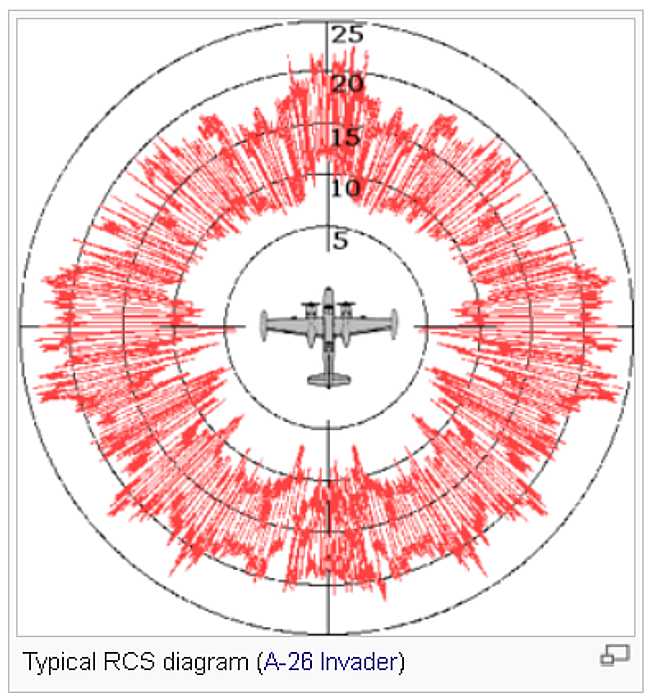
From
http://en.wikipedia.org/wiki/Radar_cross-section
The units are in dB (logarithmic power ratio), very useful in engineering.
for conversion see http://www.crownaudio.com/db-volts.htm
10 dB is a voltage ratio of 3.1, 20 dB is a voltage ratio of 10
Using the data in "Stealth" below, a reduction in reflectivity of 10 dB reduces the effective detectable range by
a factor of 1.77

"Presentation Range - 200,000 yards"
Notes on detectable range and "stealth" aircraft
(who wants his radar to spot aircraft as far away as practical)
Doubling the detectable range requires (all other things remaining the same)
increasing power by 16
target_radar_cross_section * radar_power * antenna_gain
/ range^2
reflected_power * antenna_gain / range^2
so
effective_radar_range ~ ((antenna_gain ^2) * radar_power) ^0.25
so
multiply
original power by range change
factor detection range,
if originally 128 miles
2 1.2 152
4 1.4 180
8 1.68 214
16 2.0 256
(who wants his aircraft to have low visibility to radar)
Pity the poor aircraft designer whose aircraft can be seen by a radar at 128 miles,
and is told to make the aircraft "invisible" at 8 miles.
or
reducing effective cross section by 16
So, to decrease the detection range of the aircraft by a factor of 16,
the designer/manufacturer has to decrease the reflectivity of the
aircraft by a factor of 65,536, likely to be a really major effort.
divide
original reflectivity by
range change
factor
detection range,
if originally 128 miles
2 1/1.2 106
4 1/1.4 92
8 1/1.68 76
16 1/2.0 64
256 1/4 32
4096 1/8 16
65536 1/16 8
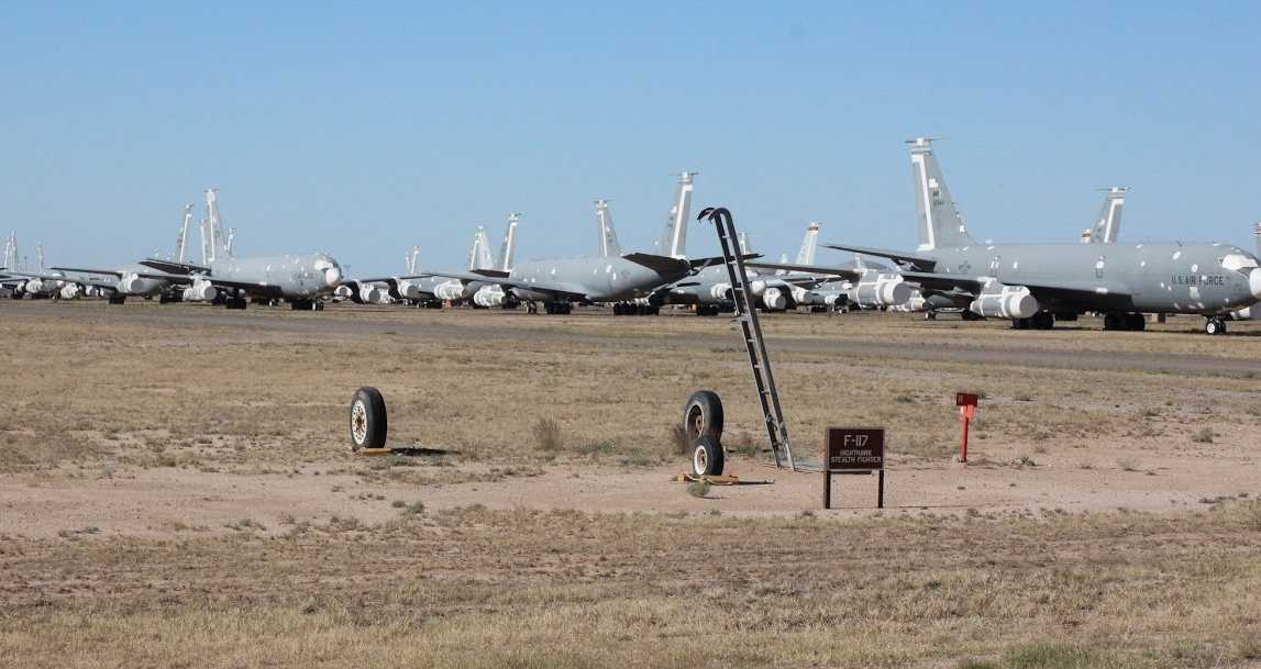
The first Stealth fighter goes to the Boneyard
;-))
From: Ron Pickinpaugh
If you really want to torment yourself, try to get current. (Items from Greg Brown)
Digital Signal Processing (DSP) in radar by Skolnik.
This must be post graduate level.
a recommended introduction
Summation: Accidental jamming was not a significant problem in Nike sites,
even when located close together as in firing ranges.
There is an Electronic Warfare organization calling itself "Old Crows"
They have a nice series of courses, available to non-members who register
at
http://www.crows.org/events/aoc-virtual-series-archive.html.
Go down that page until you find a picture of a ?B-52? bomber with
--May 1, 2014, Jamming-Techniques-WebBanner-1
--Barrage vs. False Target vs. Precision Jamming Techniques
--Presented by: Don Sedor, Sr. Systems Engineer, MacAulay-Brown
Go down the page until you find a "REGISTER" button. Click on that -
fill out the blanks, and you get to see the saved presentation.
It starts simple, and goes onto more than you want to know ;-))
Ed
It was not required training. No one else had gone. They may have had a slot and needed to send someone. I was an Acquisition Radar Operator and someone ask me and I said OK.
 I remember sitting in front of a screen simulators. These radar simulators could simulate repeaters, dropping chaff and turn back into it, spoofing, and false target jamming. We had to employ countermeasures and counter countermeasures. We had to change frequencies and watch the screen sweep for any differences in the blip on each sweep before the jamming and afterwards. We change our frequencies a lot, sometimes before the next jamming. I do not remember why but some frequencies were better for some jamming types than others. The instructors would tell you what to look for. We would look at the sweep for one blip that trailed or ahead by a hair, a new blip or blip in a different position, or brighter blip from last sweep or jamming. Speed was the game.
Don
AN/FPS-75 Alternate Battery Acquisition Radar (ABAR) & Electronic Counter Counter Measures (ECCM) Console from the point of view of the Radar Operator.
Some of the most popular types of jamming used by the ECM Specialist on enemy aircraft are:
The ECM Specialist on the aircraft and ECCM Radar Operator at the radar site play a type of electronic chess game. This game is played with very serious intent and can result in deadly consequences.
- Jamming Exercises
- Target Tracking Operations
[From the book Introduction to Radar Systems by Merrill L. Skolnik, 1980,
pages 549-550]
[From the book Introduction to Radar Systems by Merrill L. Skolnik, 1980,
page 549]
also
AOC Virtual Series Archive - interesting viewing !!
Patrick Tufts then found an almost local
(for me) copy the book
via Advanced Book Exchange.
... excellent book on the subject called "An Illustrated Guide To The
Techniques And Equipment Of Electronic Warfare" by Doug Richardson (An ARCO
Military Book) which has tons of info on that kind of thing. My copy is
pretty dated (1985) but there's probably a newer version of it by now.
There's about 20 pages on different jamming techniques and a really good
introduction explaining how radar works and all the different types of
radar. The book has plenty of pictures and diagrams, and is really easy to
understand. I highly recommend it."
and if that is not enough see
"Radar Electronic Counter-Countermeasures"
should provide more than enough.
http://www.valuewalk.com/2015/10/sophisticated-electronic-warfare-giving-russia-edge/
from http://fullafterburner.weebly.com/next-gen-weapons/electronic-warfare-deception-jamming
5/26/2018
The ability of a target aircraft to carry and launch a missile to follow down
your radar beam to your radar (and you) was just a future possibility in 1956.
To put a useful radar tracker into a missile small enough
to be handy is an interesting design and production challenge.
The actual category of weapons is
called ARMs (Antiradiation Missile) while the HARM (High Speed
Antiradiation Missile) refers to a specific weapon, the AGM-88.
ARMS were first used in the Vietnam War in Mar 1966 by Wild Weasel 1
(F-100F) aircraft carrying the AGM-45 Shrike, the first ARM in the US
inventory.
I just read the update, at the bottom you assert that the HARM is the
best ARM around ,that is only partly correct. You are correct if you
saying it is the best American ARM around. The best ARM around is the
British aerospace ALARM, not is it more modern, it is half the weight of
a HARM and is flexible since if it does not immediately detect its
target ,it climbs to 70000Ft and deploys a drogue chute. It can stay in
this mode for 15 minutes, if detects the target during this period it
cuts lose and literally drops in detonating when it is beside the target
in a vertical dive.
Various groups use measurements of historical or practical
significance. Examples are the jeweler's use the "carat" for weight and American's
use of the old "English" system of measurements.
(*) Units that only scientists or engineers love.
unit
S.I. (mks, metric) name
an "English" name
Artillery name
length
meter yard yard
volume
liter gallon gallon
force
newton(*) pound pound
mass
kilogram
slug(*) .
plane angle
radian degree or radian(*) mil(**) (equals milliradian)
time
second second second
temperature
degree Celsius or Kelvin(*) degree Fahrenheit
degree Fahrenheit
(**) The angle included by 1 unit at a range of 1000 units. 1 mil equals about 0.0573 degrees.
This strange sounding unit is very handy in aiming and estimating errors in
gun artillery and missiles. An azimuth error of 1 mil at a range of 25,000 yards
is a miss by 25 yards. A tracking radar pointing error of 0.1 mils (0.00573 degrees)
at range of 132,000 yards (75 miles) yields a "miss" of 13.2 yards. (A Nike warhead
exploding 13 yards from a flying aircraft will instantly turn that aircraft into
a falling pile of junk.)
"The only change that I can see would be that we seldom use yards any more,
but describe that unit of measure in terms of meters.
That ties in with our use of military grid overlays on maps
which are done in meters and kilometers.
Altitude is still done in thousands of feet, just like commercial airliners use,
"Ladies and gentlemen, our cruising altitude today will be 30,000 feet."
Mils are still used in the artillery as a more precise measurement than
degrees, although degrees are used also. We still use pounds and gallons for measurement."
J.P.Moore found this:http://www.bts.gov/NTL/DOCS/3910-3a.html
If you have comments or suggestions, Send e-mail
to Ed Thelen
Return to home page,
Goto Next Section
Return to beginning of Nike Radars
Updated September, 2022
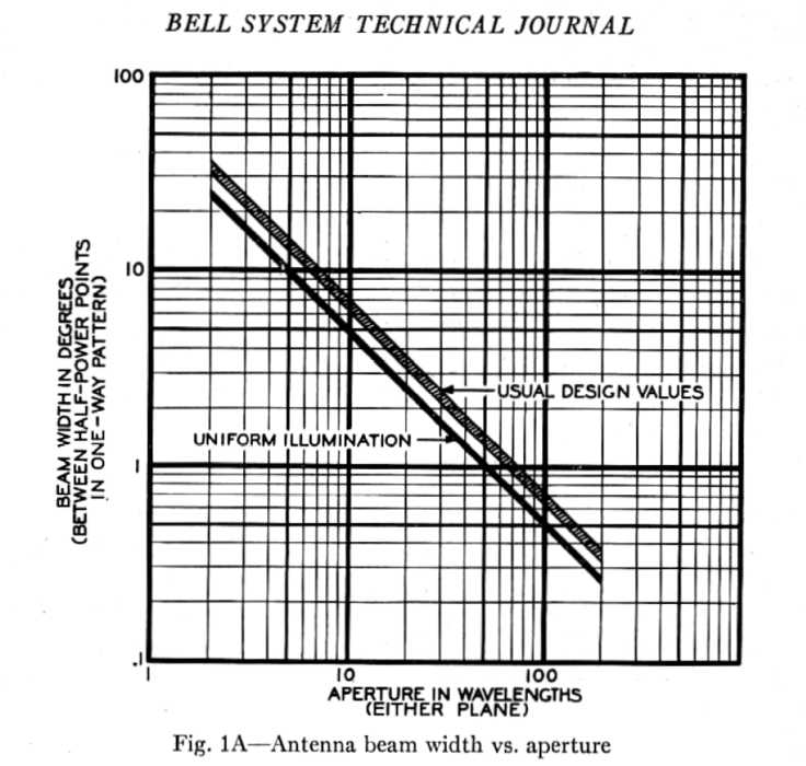
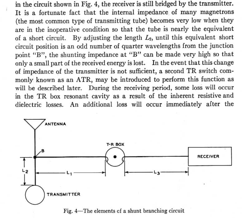
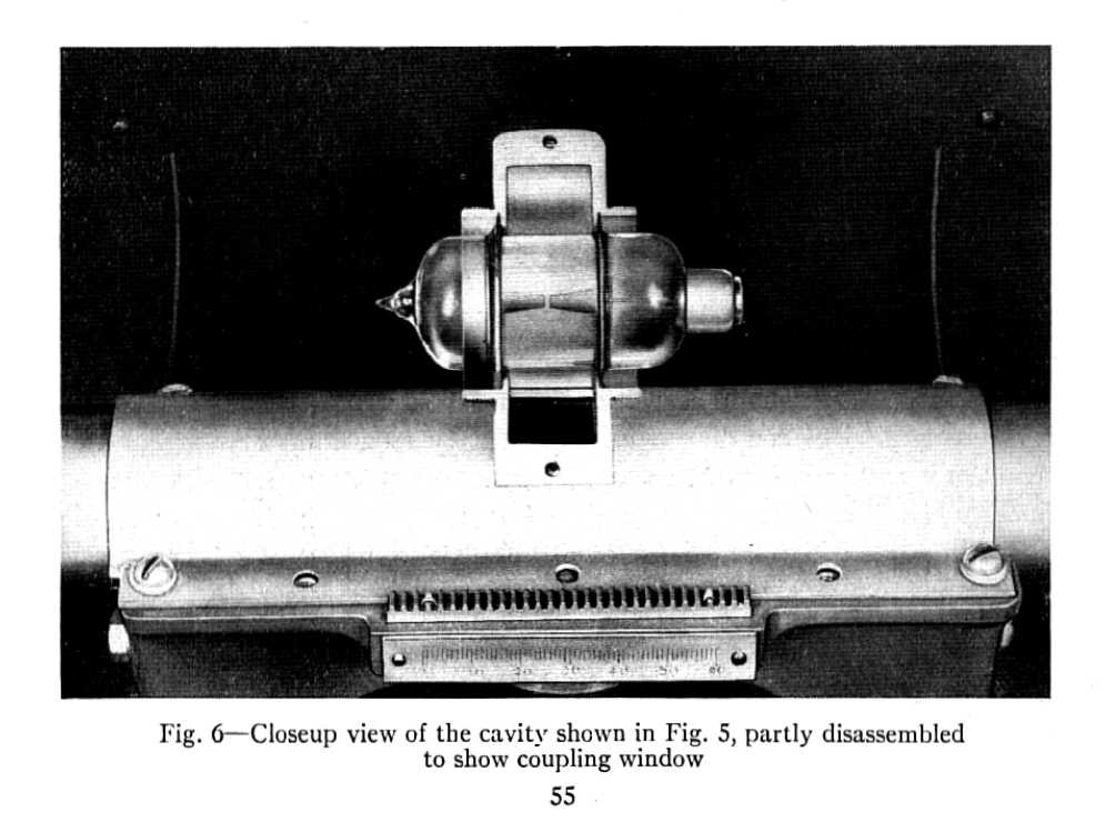
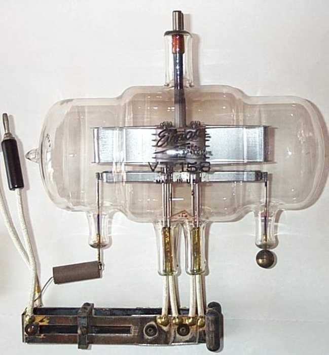
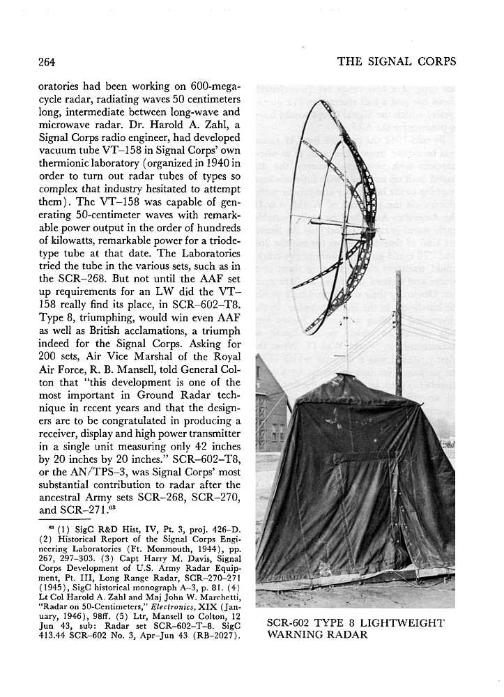
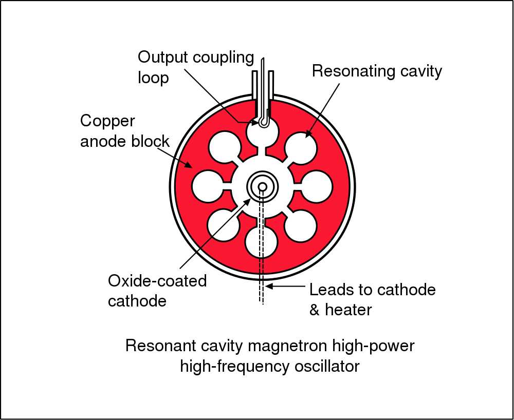
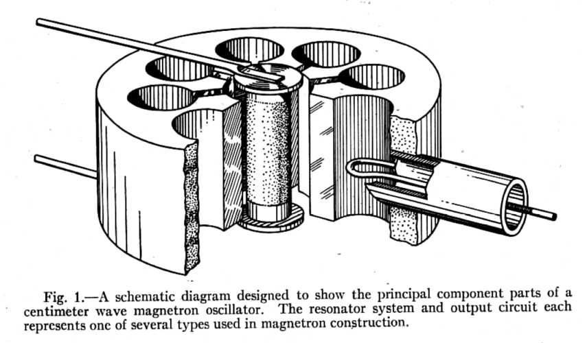
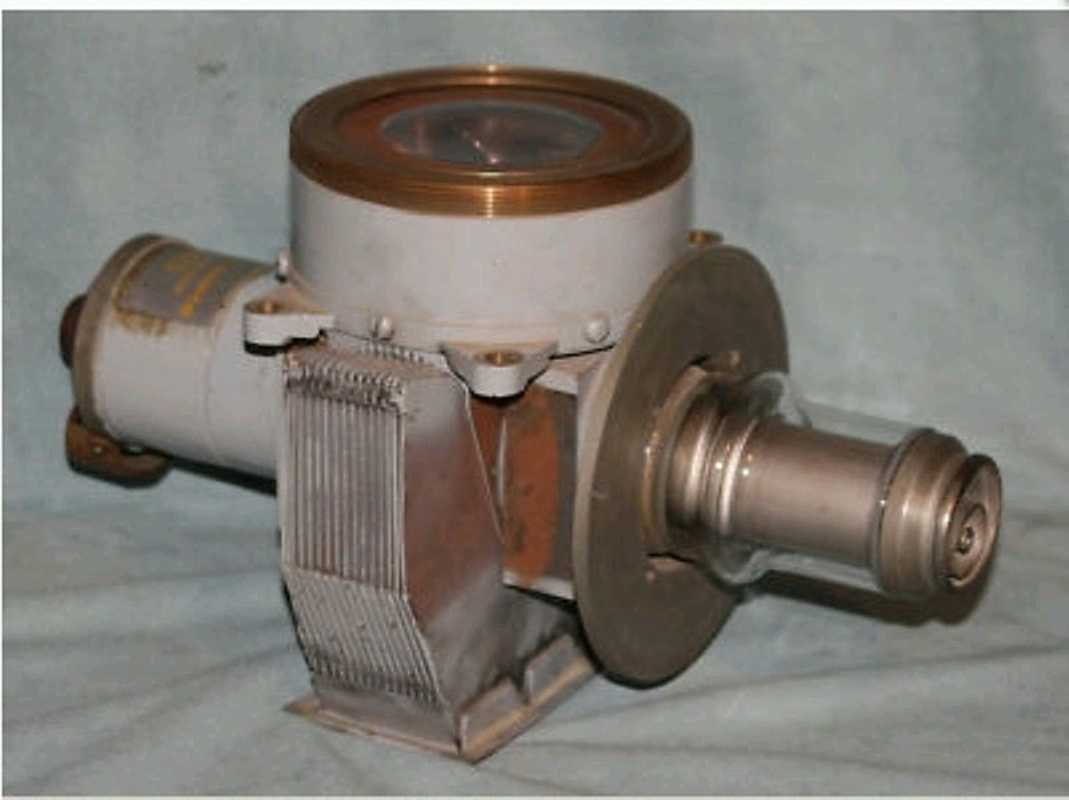
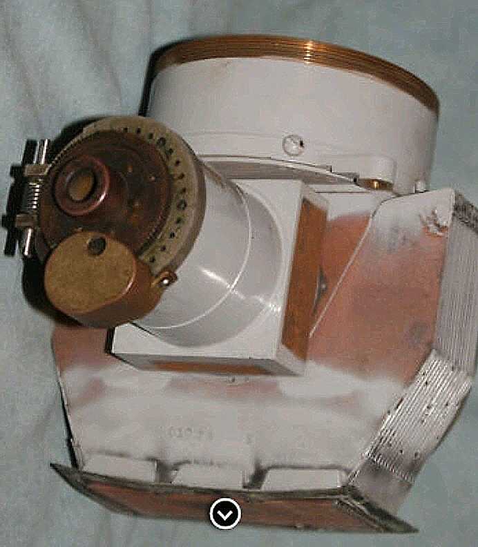
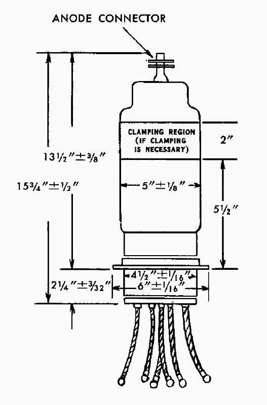
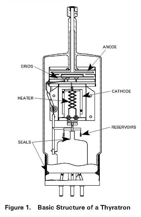
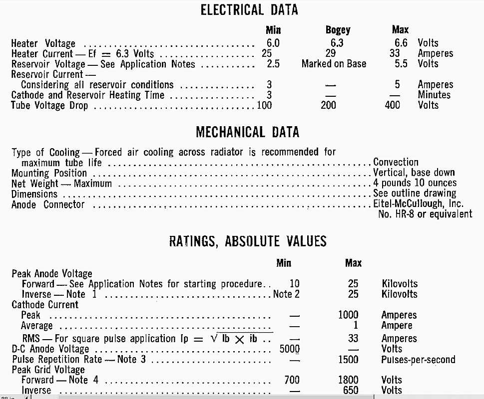

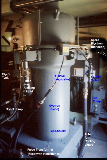 powerful klystron